2.3 — Cournot Competition
ECON 316 • Game Theory • Fall 2021
Ryan Safner
Assistant Professor of Economics
safner@hood.edu
ryansafner/gameF21
gameF21.classes.ryansafner.com
Models of Oligopoly
Three canonical models of Oligopoly
- Bertrand competition
- Firms simultaneously compete on price
- Cournot competition
- Firms simultaneously compete on quantity
- Stackelberg competition
- Firms sequentially compete on quantity
Cournot Competition
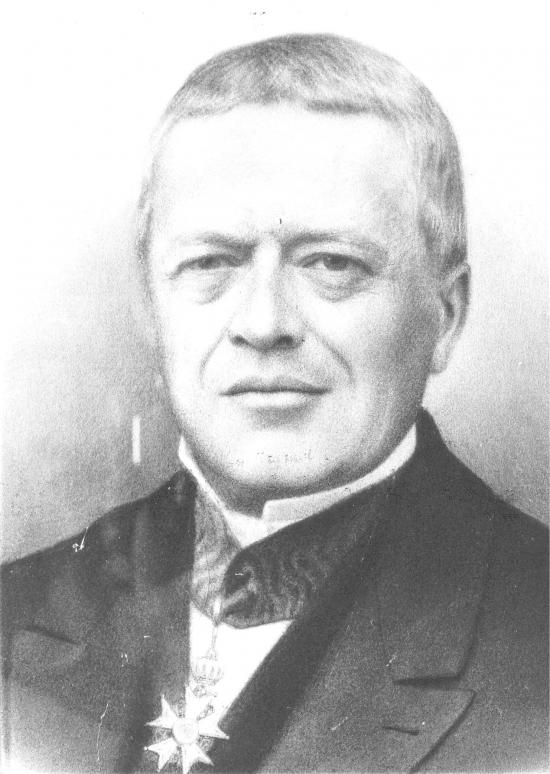
Antoine Augustin Cournot
1801-1877
"Cournot competition": two (or more) firms compete on quantity to sell the same good
Firms set their quantities simultaneously
Firms' joint output determines the market price faced by all firms
Cournot Competition: Mechanics
Suppose two firms (1 and 2), each have an identical constant cost MC(q)=AC(q)=c
Firm 1 and Firm 2 simultaneously set quantities, q1 and q2
Total market demand is given by
P=a−bQQ=q1+q2

Cournot Competition: Mechanics
- Firm 1's profit is given by:
π1=q1(P−c)π1=q1(a−b(q1+q2)−c)
And, symmetrically same for firm 2
Note each firm's profits depend (in part) on the outputs of the other firm!

Residual Demand
Consider each the demand each firm faces to be a residual demand
e.g. for firm 1
p=a−b(q1+q2)p=(a−bq2)⏟intercept−b⏟slopeq1
Firm 2 will produce some amount, q2.
Firm 1 takes this as given, to find its own residual demand
- Intercept: a−bq2
- Slope: b (in front of q1)
Residual Demand
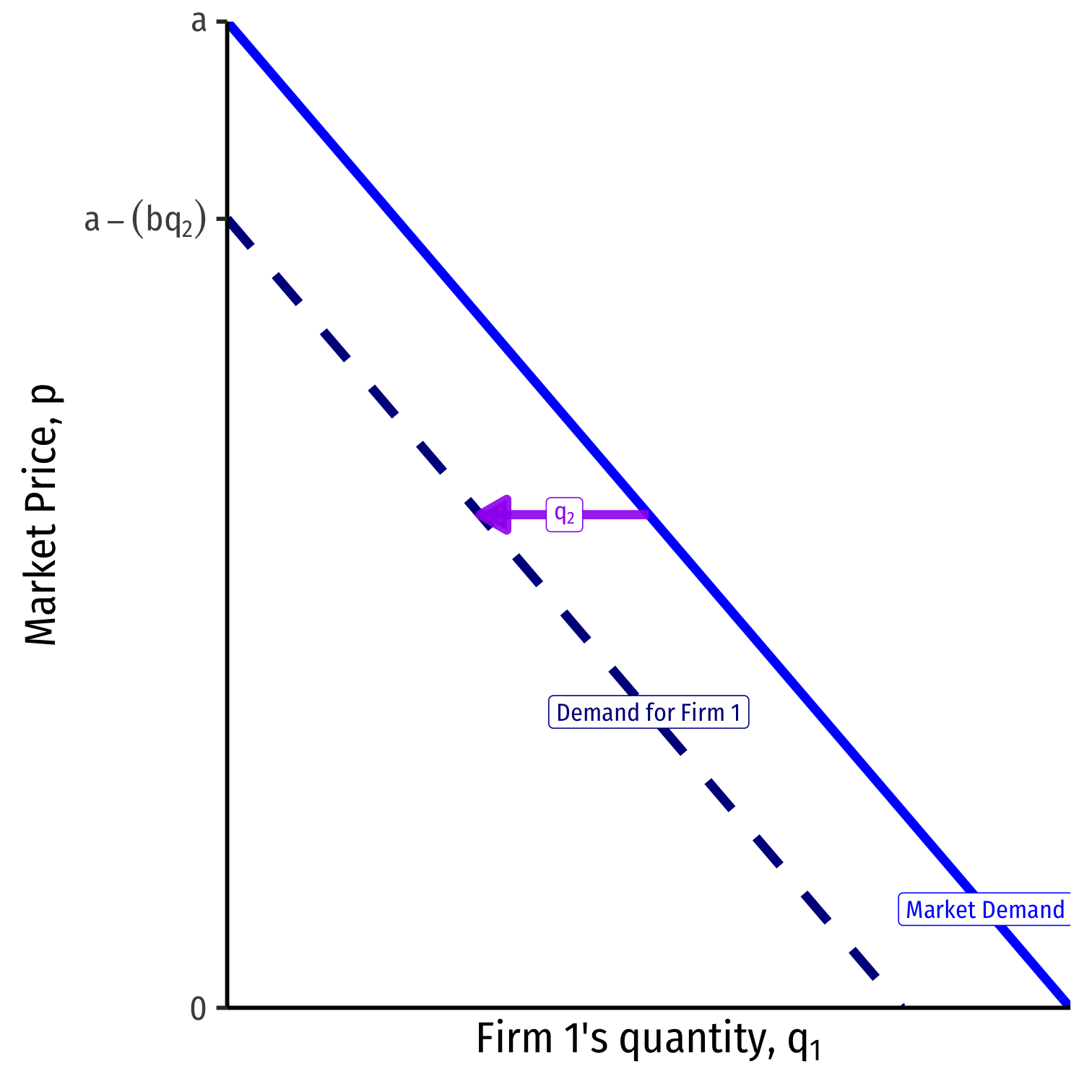
Firm 2 will produce some amount q2
Firm 1 will take this as a given, a constant
Firm 1's choice variable is q1, given q2
Cournot Competition: Example
Example: Assume Saudi Arabia (sa) and Iran (i) are the only two oil producers, each with a constant MC=AC=20. The market (inverse) demand curve is given by: P=200−3QQ=qsa+qi
Cournot Competition: Example
Example: Assume Saudi Arabia (sa) and Iran (i) are the only two oil producers, each with a constant MC=AC=20. The market (inverse) demand curve is given by: P=200−3QQ=qsa+qi
P=200−3qsa−3qi
Cournot Competition: Example
P=200−3qi⏟intercept−3qsa
- Firms maximize profit (as always), by setting q∗:MR(q)=MC(q)
Cournot Competition: Example
P=200−3qi⏟intercept−3qsa
Firms maximize profit (as always), by setting q∗:MR(q)=MC(q)
Solve for Saudi Arabia
- Take qi as given, a constant
- Recall MR is twice the slope of demand
Cournot Competition: Example
P=200−3qi⏟intercept−3qsa
Firms maximize profit (as always), by setting q∗:MR(q)=MC(q)
Solve for Saudi Arabia
- Take qi as given, a constant
- Recall MR is twice the slope of demand
MRsa=200−3qi−6qsa
Cournot Competition: Example
Solve for q∗ for each firm (where MR(q)=MC(q)), we derive each firm's reaction function or best response function to the other firm's output
Symmetric marginal costs and marginal revenues
Cournot Competition: Example
Solve for q∗ for each firm (where MR(q)=MC(q)), we derive each firm's reaction function or best response function to the other firm's output
Symmetric marginal costs and marginal revenues
q∗sa=30−0.5qiq∗i=30−0.5qsa
Saudi Arabia's Reaction Curve
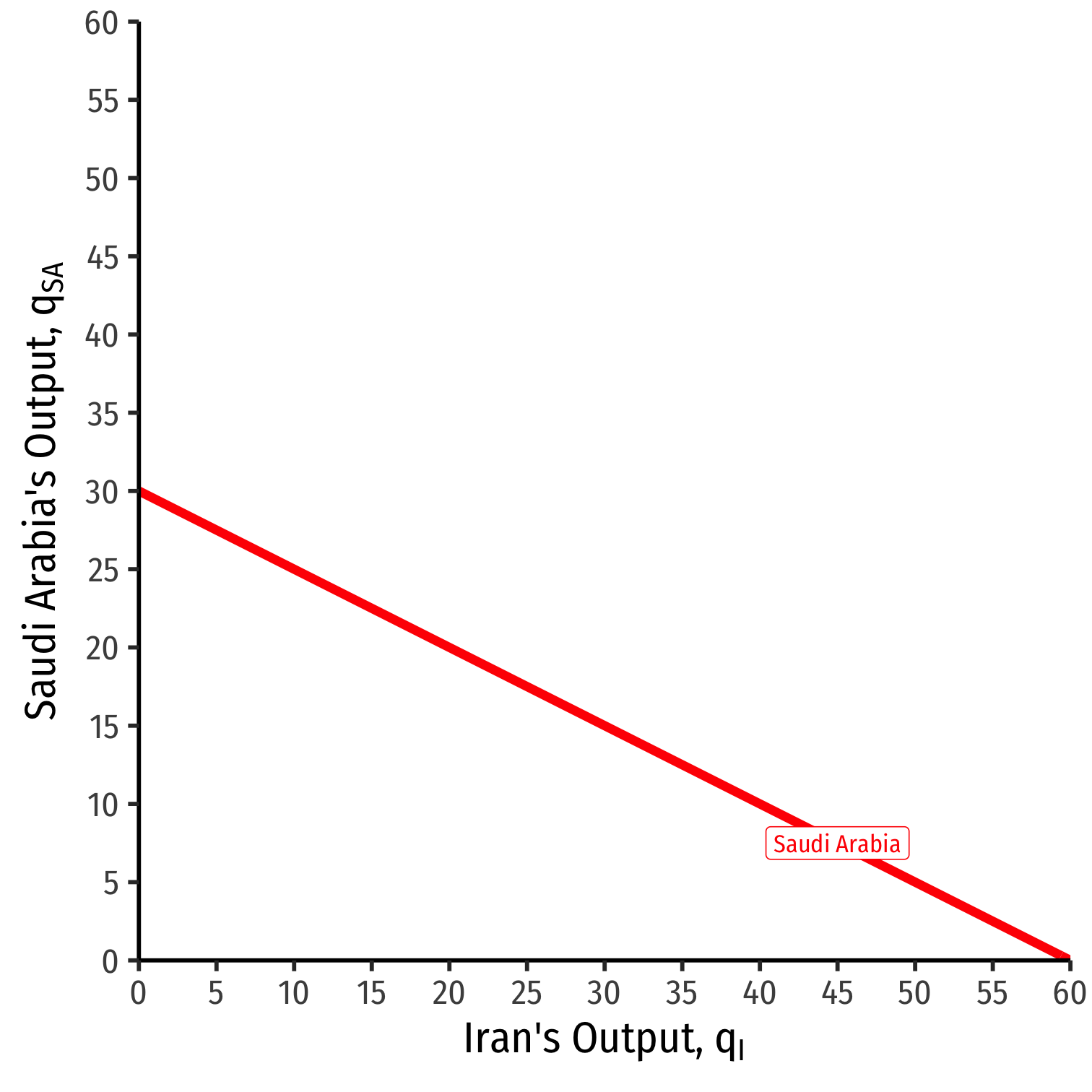
We can graph Saudi Arabias's reaction curve to Irans's output
Saudi Arabia's Reaction Curve
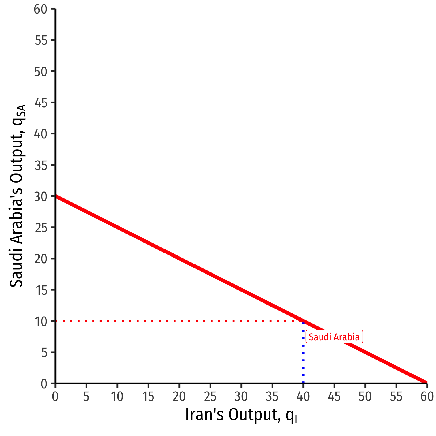
We can graph Saudi Arabias's reaction curve to Irans's output
- e.g. if Iran produces 40, Saudi Arabia's best response is 10
Saudi Arabia's Reaction Curve
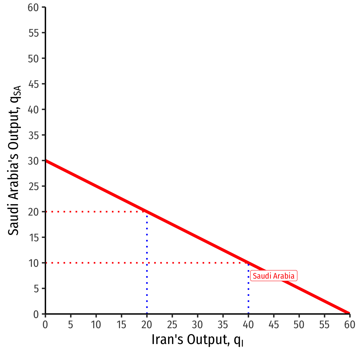
We can graph Saudi Arabias's reaction curve to Irans's output
- e.g. if Iran produces 40, Saudi Arabia's best response is 10
- e.g. if Iran produces 20, Saudi Arabia's best response is 20
Iran's Reaction Curve
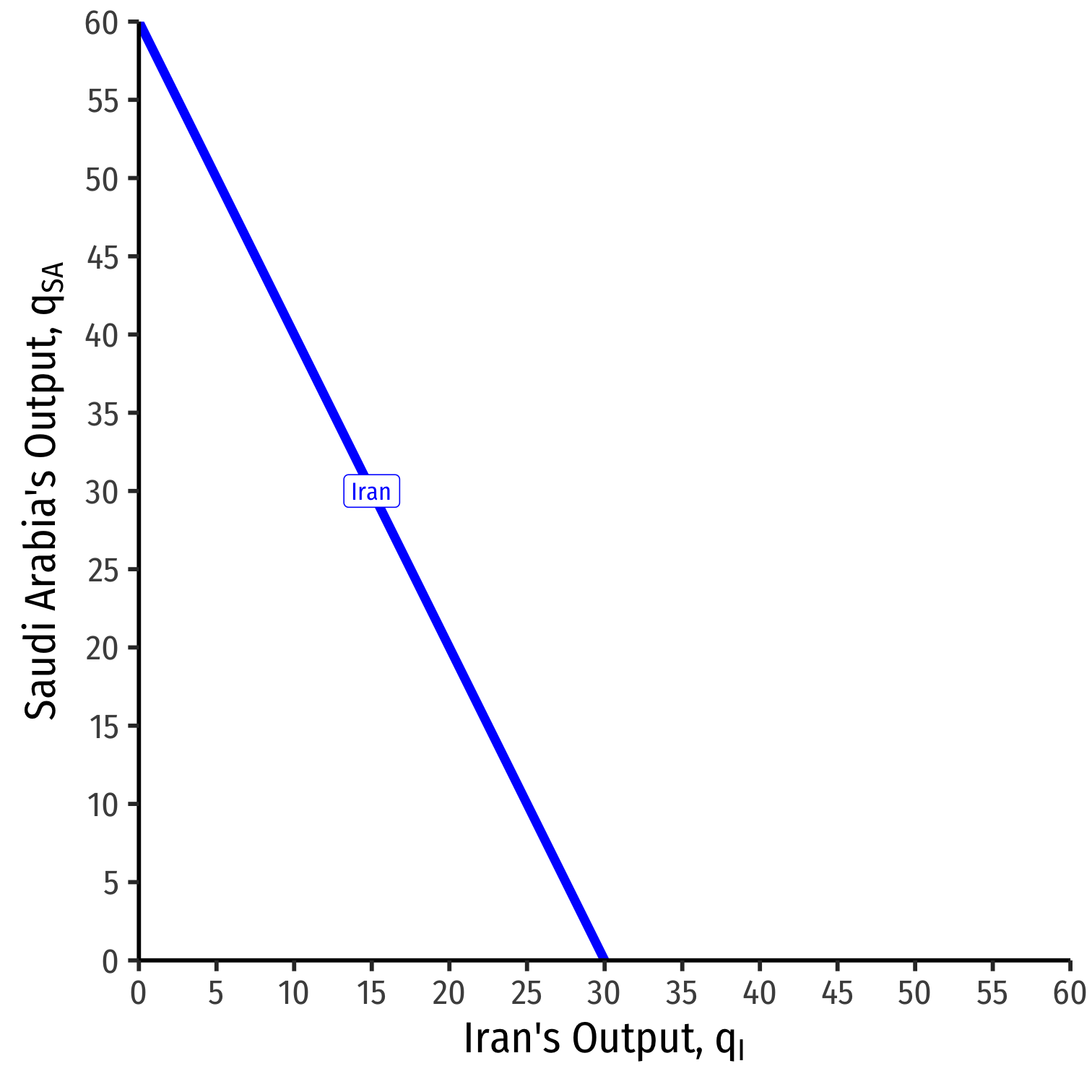
We can graph Iran's reaction curve to Saudi Arabia's output
Iran's Reaction Curve
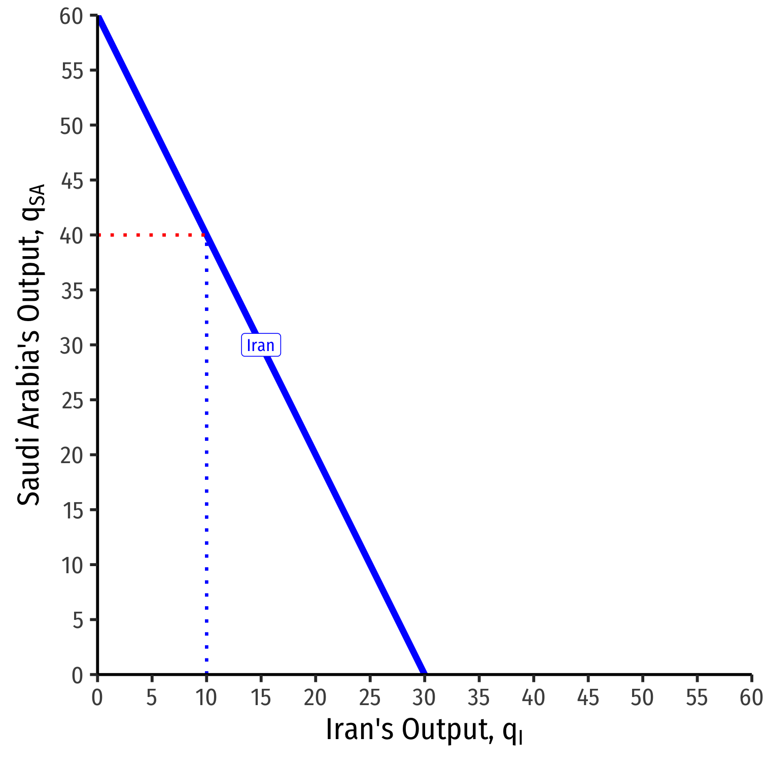
We can graph Iran's reaction curve to Saudi Arabia's output
- e.g. if Saudi Arabia produces 40, Iran's best response is 10
Iran's Reaction Curve
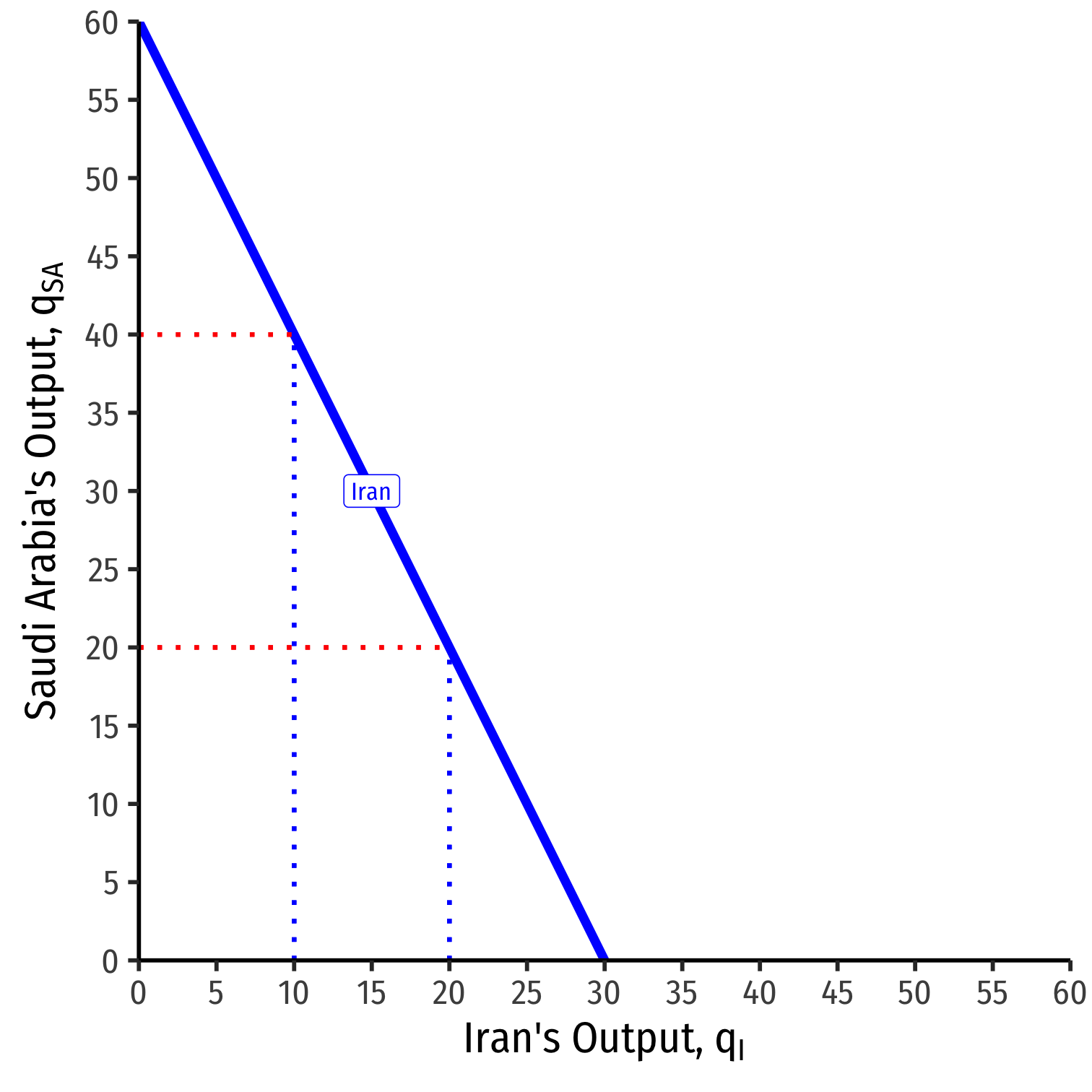
We can graph Iran's reaction curve to Saudi Arabia's output
- e.g. if Saudi Arabia produces 40, Iran's best response is 10
- e.g. if Saudi Arabia produces 20, Iran's best response is 20
Cournot-Nash Equilibrium, Graphically
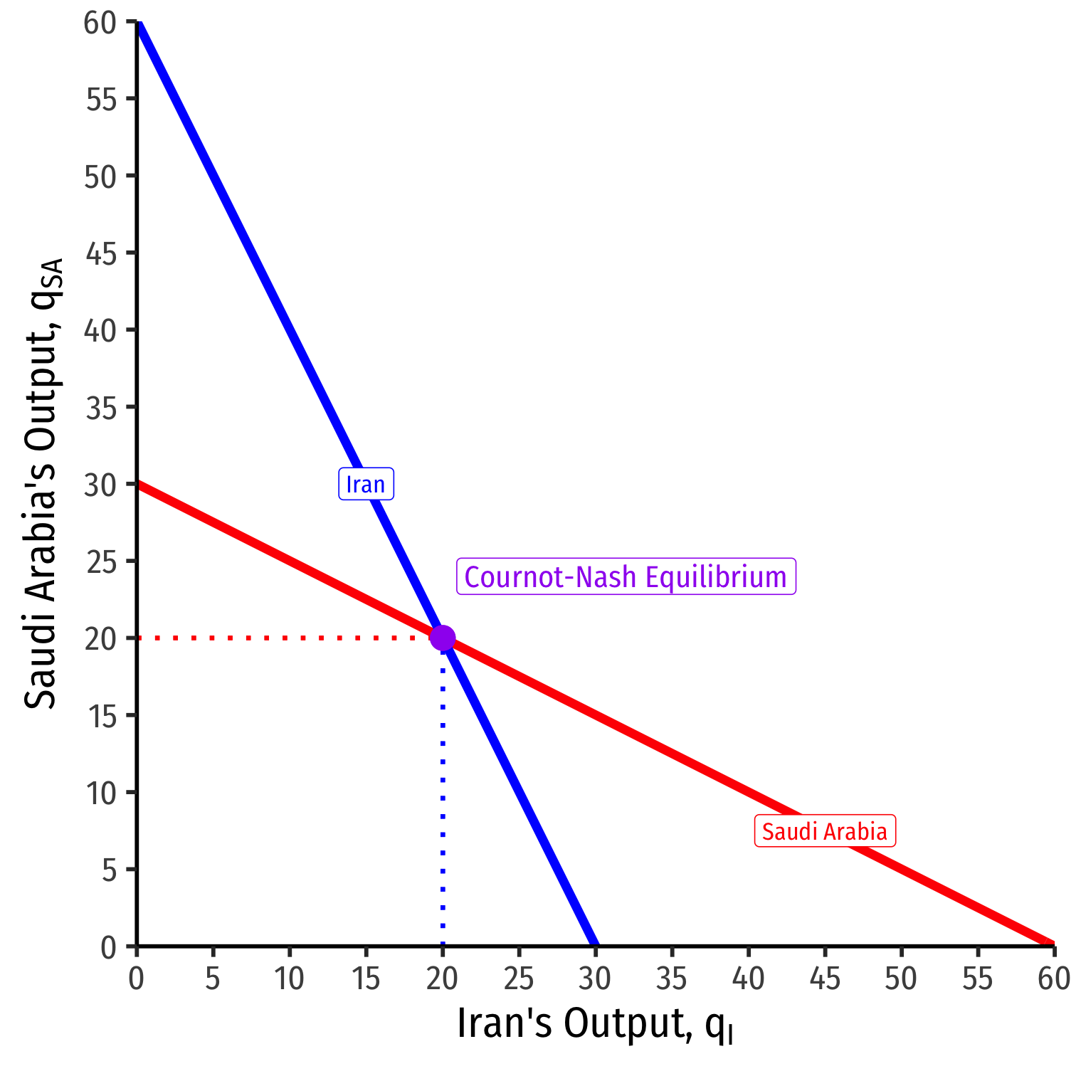
Combine both curves on the same graph
Cournot-Nash Equilibrium: (20,20)
- Where both reaction curves intersect
Both are playing mutual best response to one another
Cournot-Nash Equilibrium, Algebraically
- Cournot-Nash Equilibrium algebraically: plug one firm's reaction function into the other's
Cournot-Nash Equilibrium, Algebraically
- Cournot-Nash Equilibrium algebraically: plug one firm's reaction function into the other's
q∗sa=30−0.5qiq∗i=30−0.5qsa
Cournot-Nash Equilibrium, Algebraically
- Cournot-Nash Equilibrium algebraically: plug one firm's reaction function into the other's
q∗sa=30−0.5qiq∗i=30−0.5qsa
- The market demand again was
P=200−3qsa−3qi
Cournot-Nash Equilibrium, Algebraically
- Both countries produce 20
Cournot-Nash Equilibrium, Algebraically
- Both countries produce 20
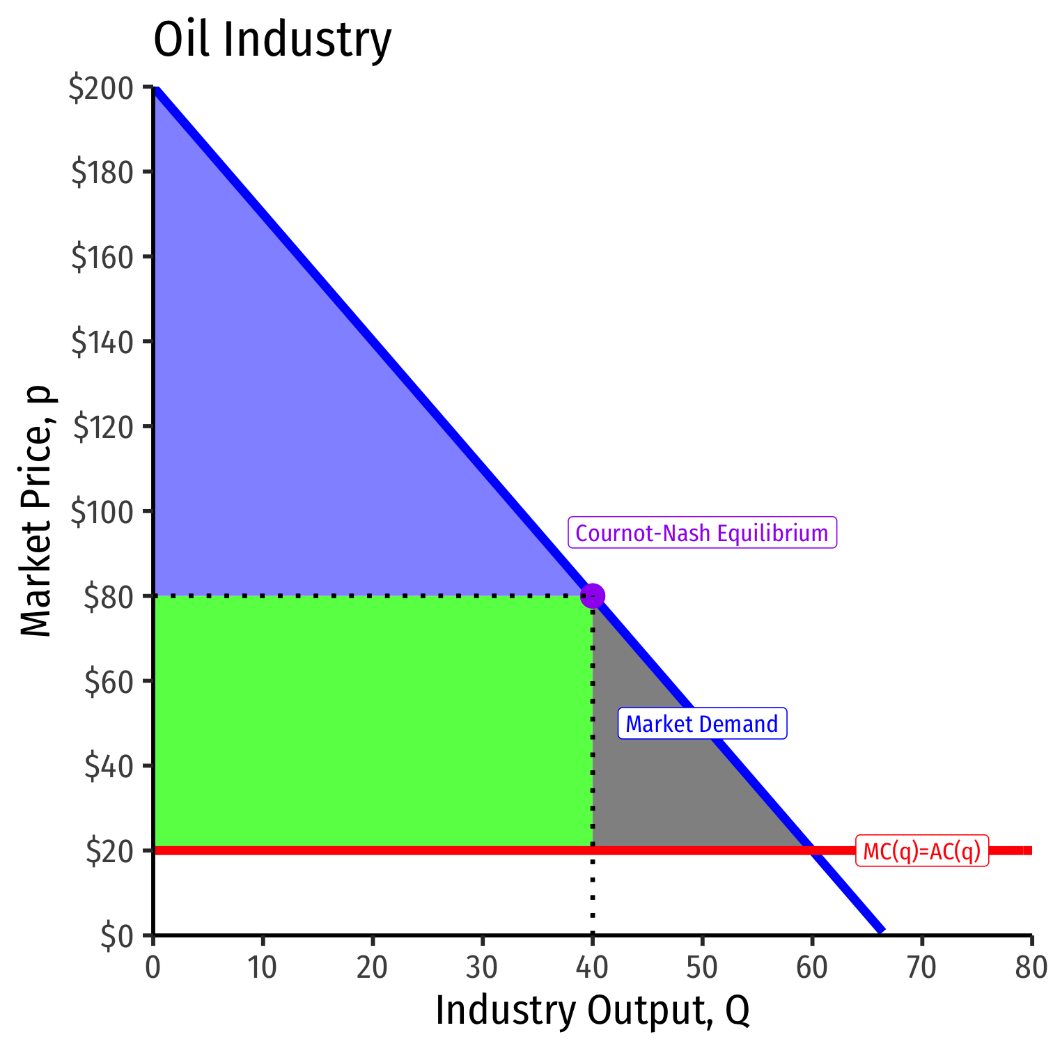
P=200−3(20)−3(20)P=$80
Cournot-Nash Equilibrium, Algebraically
- Both countries produce 20
P=200−3(20)−3(20)P=$80
- Find profit for each country:
Cournot-Nash Equilibrium, Algebraically
- Both countries produce 20
P=200−3(20)−3(20)P=$80
- Find profit for each country:
πsa=qsa(P−c)πsa=20(80−20)πsa=1,200
- Symmetrically for Iran, πi=1,200
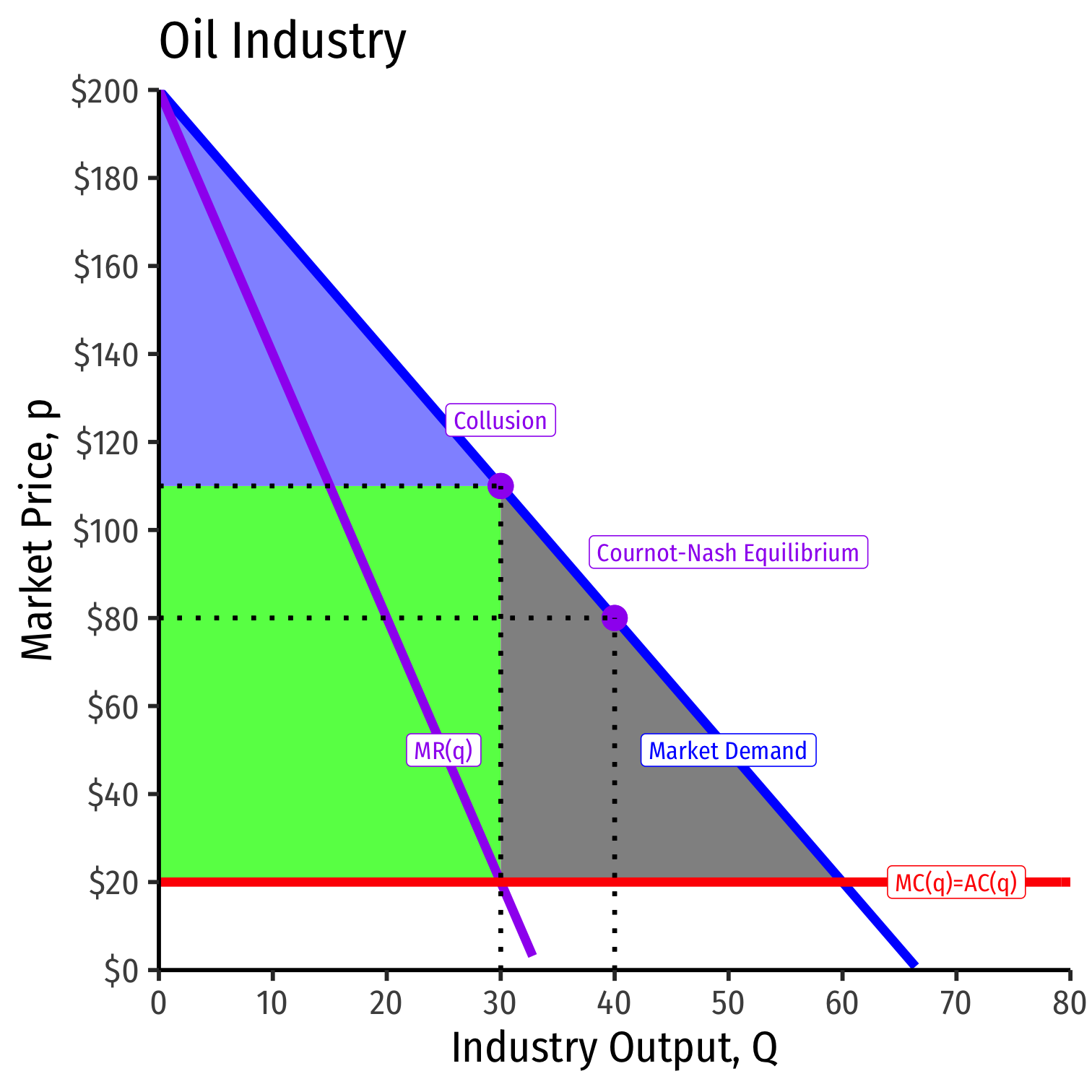
Cournot-Nash Equilibrium, The Market
Cournot Collusion
- Suppose now both firms collude to act like a monopolist, who sets the entire market:
MR=MC200−6Q=2030=Q∗
Cournot Collusion
- Suppose now both firms collude to act like a monopolist, who sets the entire market:
MR=MC200−6Q=2030=Q∗
- The monopoly price will then be:
P=200−3(30)P=$110
Cournot Collusion
- Suppose now both firms collude to act like a monopolist, who sets the entire market:
MR=MC200−6Q=2030=Q∗
- The monopoly price will then be:
P=200−3(30)P=$110
- Total profit will then be:
Π=30(110−20)=$2,700
with $1,400 going to each firm
Cournot Collusion
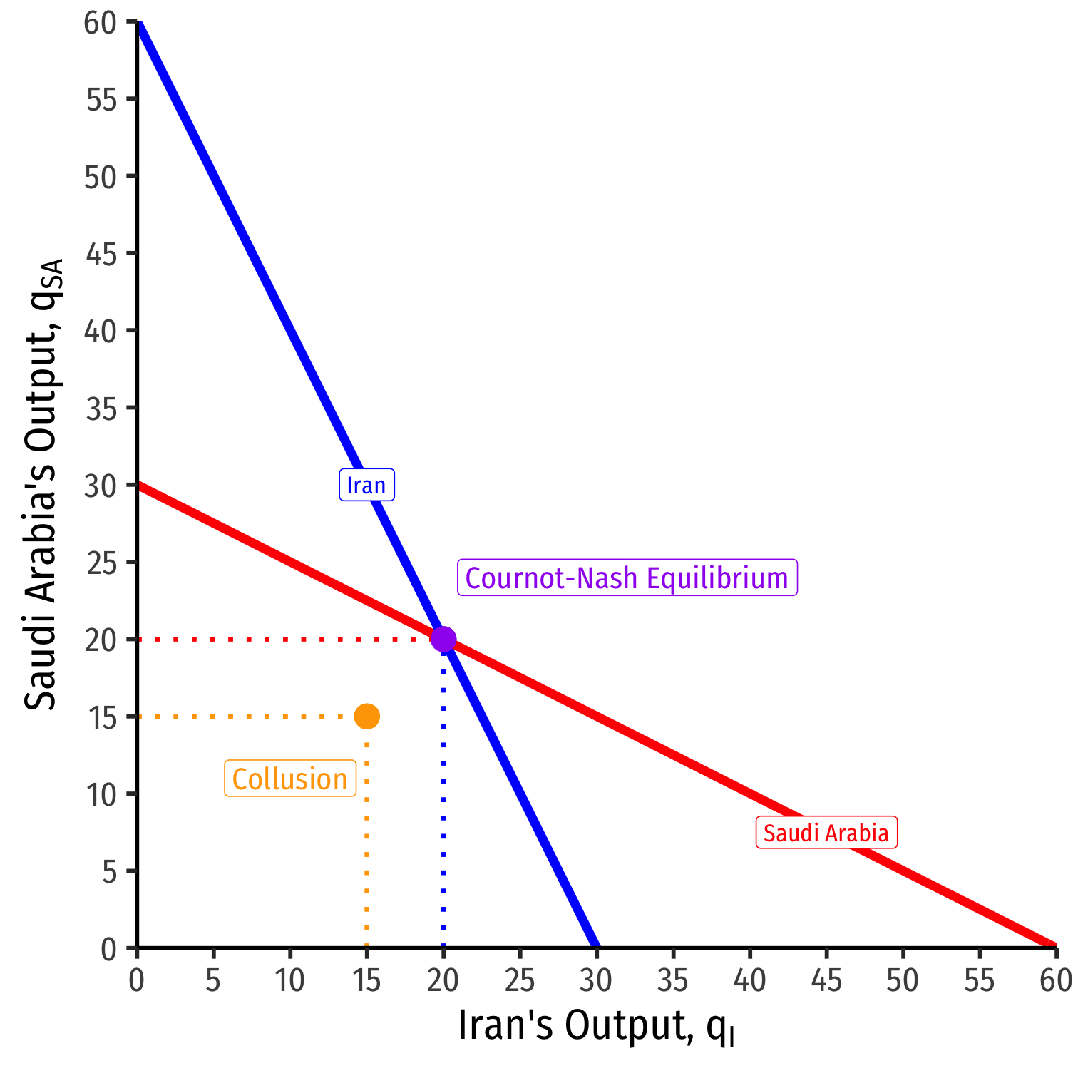
Cournot Competition: each firm produces 20 and earns $1,200
Cournot Collusion: each firm produces 15 and earns $1,400
Cournot Collusion

Cournot Competition: each firm produces 20 and earns $1,200
Cournot Collusion: each firm produces 15 and earns $1,400
But is collusion a Nash equilibrium?
Cournot Collusion
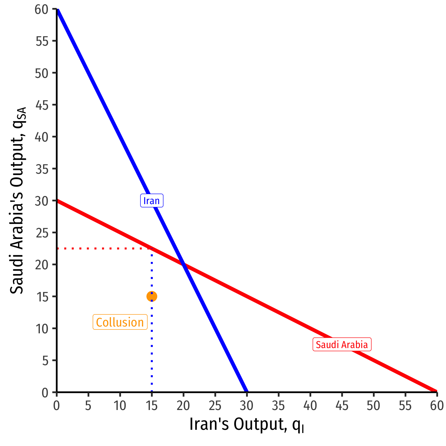
Read either firm's reaction curve at the collusive outcome
Suppose Saudi Arabia knows Iran is producing 15 (as per the cartel agreement)
Saudi Arabia's best response to Iran's 15 is to produce 22.5
Cournot Collusion
- This would bring market price to
P=200−3qsa−3qiP=200−3(22.5)−3(15)P=$87.50
Cournot Collusion
- This would bring market price to
P=200−3qsa−3qiP=200−3(22.5)−3(15)P=$87.50
- Saudi Arabia's profit would be:
πsa=qsa(P−c)πsa=22.5(87.50−20)πsa=$1,518.75
Cournot Collusion
- This would bring market price to
P=200−3qsa−3qiP=200−3(22.5)−3(15)P=$87.50
- Saudi Arabia's profit would be:
πsa=qsa(P−c)πsa=22.5(87.50−20)πsa=$1,518.75
- Iran's profit would be:
πi=qi(P−c)πi=15(87.50−20)πi=$712.50
Cournot Collusion, The Market
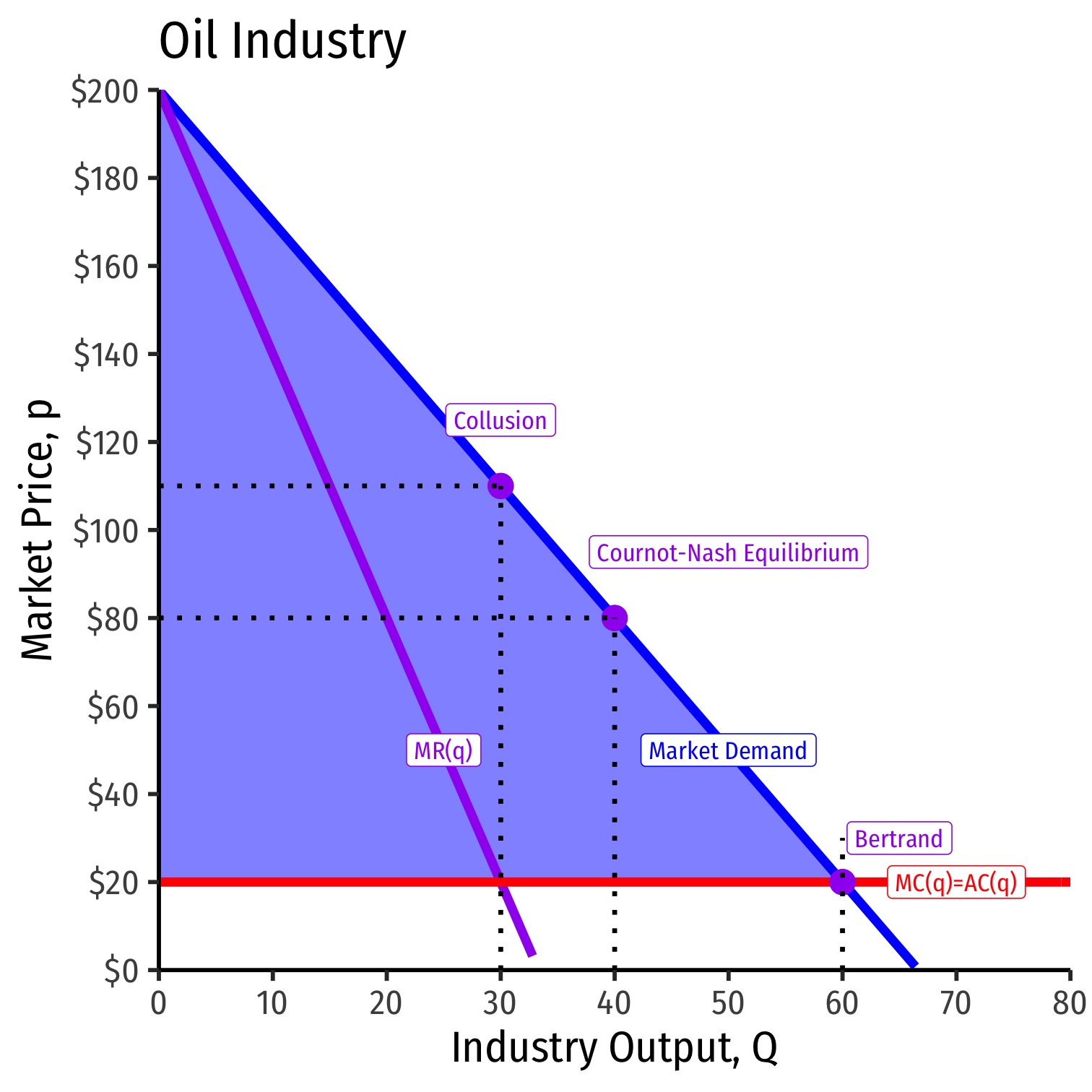
Bertrand Competition for our Example
Imagine Bertrand competition between Saudi Arabia and Iran instead (price competition)
Nash equilibrium: Firms will set P=MC, so:
P=MC200−3Q=20Q=60
Both countries split demand equally, each selling 30 units
Profit for both countries would be 0, since P=MC
Bertrand Competition, The Market
Cournot vs. Bertrand Competition
| Type | Output | Price | Profits |
|---|---|---|---|
| Collusion | 30 | $110 | $2,700 |
| Cournot | 40 | $80 | $2,400 |
| Bertrand | 60 | $20 | $0 |
Cournot vs. Bertrand Competition
| Type | Output | Price | Profits |
|---|---|---|---|
| Collusion | 30 | $110 | $2,700 |
| Cournot | 40 | $80 | $2,400 |
| Bertrand | 60 | $20 | $0 |
- Output: Qm<Qc<Qb
- Market price: Pb<Pc<Pm
- Profit: πb=0<πc<πm
Where subscript m is monopoly (collusion), c is Cournot, b is Bertrand
Cournot Competition, You Try
Example: Suppose Firm 1 and Firm 2 have a constant MC=AC=8. The market (inverse) demand curve is given by:
P=200−2QQ=q1+q2
Find the Cournot-Nash equilibrium output and profit for each firm.
Find the output and profit for each firm if the two were to collude.
Find the price and output if the two were to compete on price instead of quantity.
Cournot Competition

Antoine Augustin Cournot
1801-1877
Cournot Theorem: as the number of firms (N) in the market increases, market output Nq goes to the competitive level, and price converges to c.
- Assuming no fixed costs, and an identical constant marginal cost for firms
More (fewer) firms reduce (increase) market distortions from market power
Cournot Competition: Implications

Antoine Augustin Cournot
1801-1877
- See some visualizations I made:
Major implications from Cournot:
As ↑ number of firms: ↑Q, ↓p, ↓π, ↑CS, ↓DWL (closer to perfect competition)
If a firm has lower costs than others, it earns greater profit. Firms will want to lower their own costs OR raise rivals' costs (same effect)
Cournot Competition on Moblab

Cournot Competition on Moblab
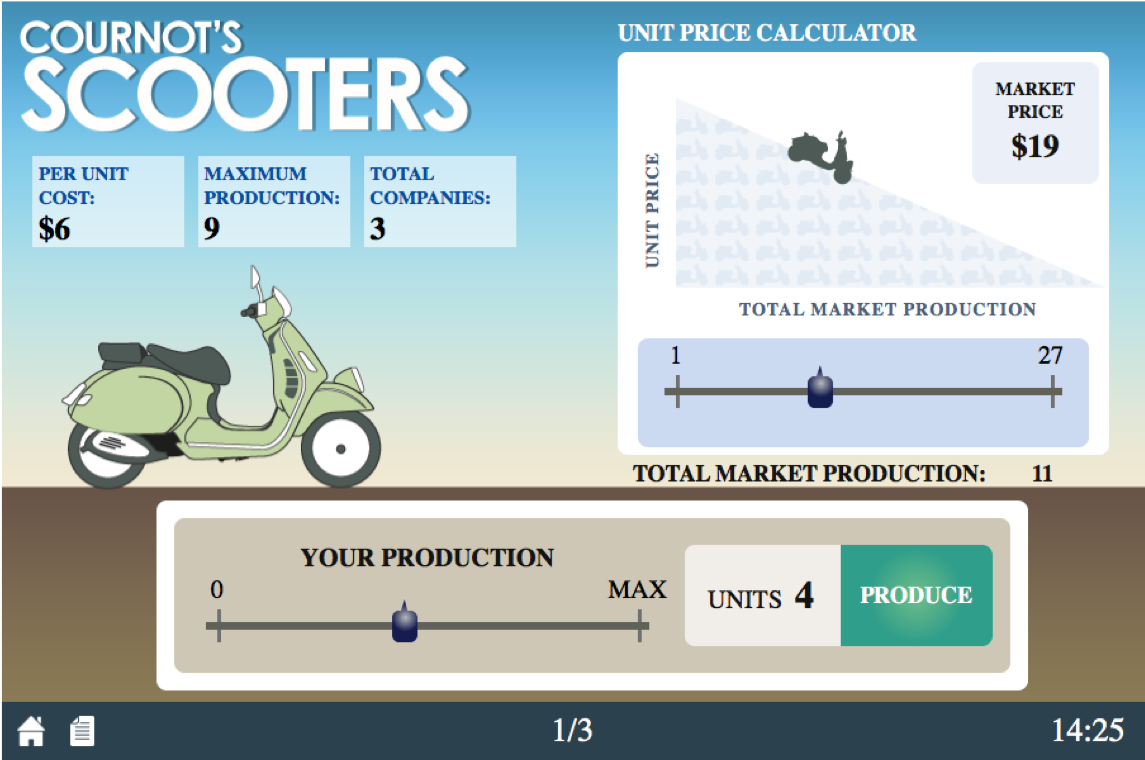
- Each of you is a firm selling identical scooters
- Each season, each firm chooses its quantity to produce
- You pay a cost for each you produce (identical across all firms)
- Market price depends on total industry output
- More total output ⟹ lower market price
- Market price is revealed after all firms have chosen their output

Cournot Competition on Moblab
- We will play 4 times:
- You are the only firm (monopoly)
- You will be matched with another firm (duopoly)
- You will be matched with 2 other firms (triopoly)
- The entire class is competing in the same market (N=10)
- Each instance will have 3 rounds
