4.4 — Incomplete & Asymmetric Info.
ECON 316 • Game Theory • Fall 2021
Ryan Safner
Assistant Professor of Economics
safner@hood.edu
ryansafner/gameF21
gameF21.classes.ryansafner.com
Information in Games
Information
Perfect information: all players know the rules and all possible strategies, payoffs, and move history of other players
Common knowledge assumption: Player 1 knows that Player 2 knows that Player 1 knows that ...

Information
Imperfect information: players all know the game, but don't know what other players are choosing
- “Strategic uncertainty”
- Seen as simultaneous games
Incomplete information: players don't have all the information about the game
- “External uncertainty”
- Who the other players are, what payoffs are, etc.

Simultaneous Games and Imperfect Information
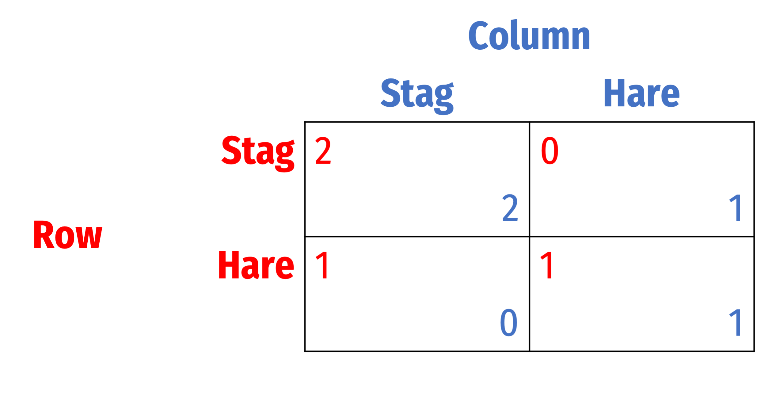
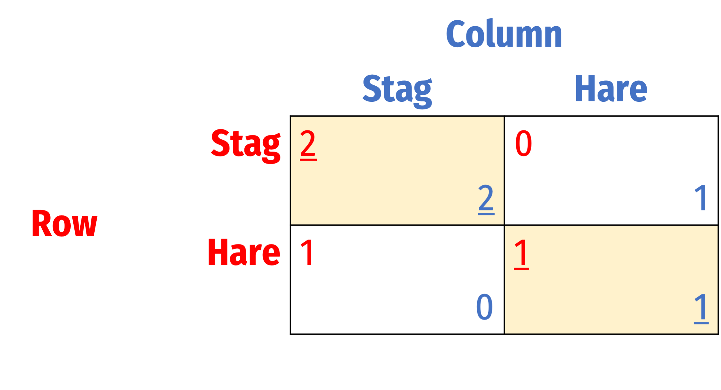
Let’s consider the simultaneous-move Stag Hunt in strategic form
We can't model this as an extensive form game with perfect information
- Each player doesn’t know what the other chose
Simultaneous Games and Imperfect Information
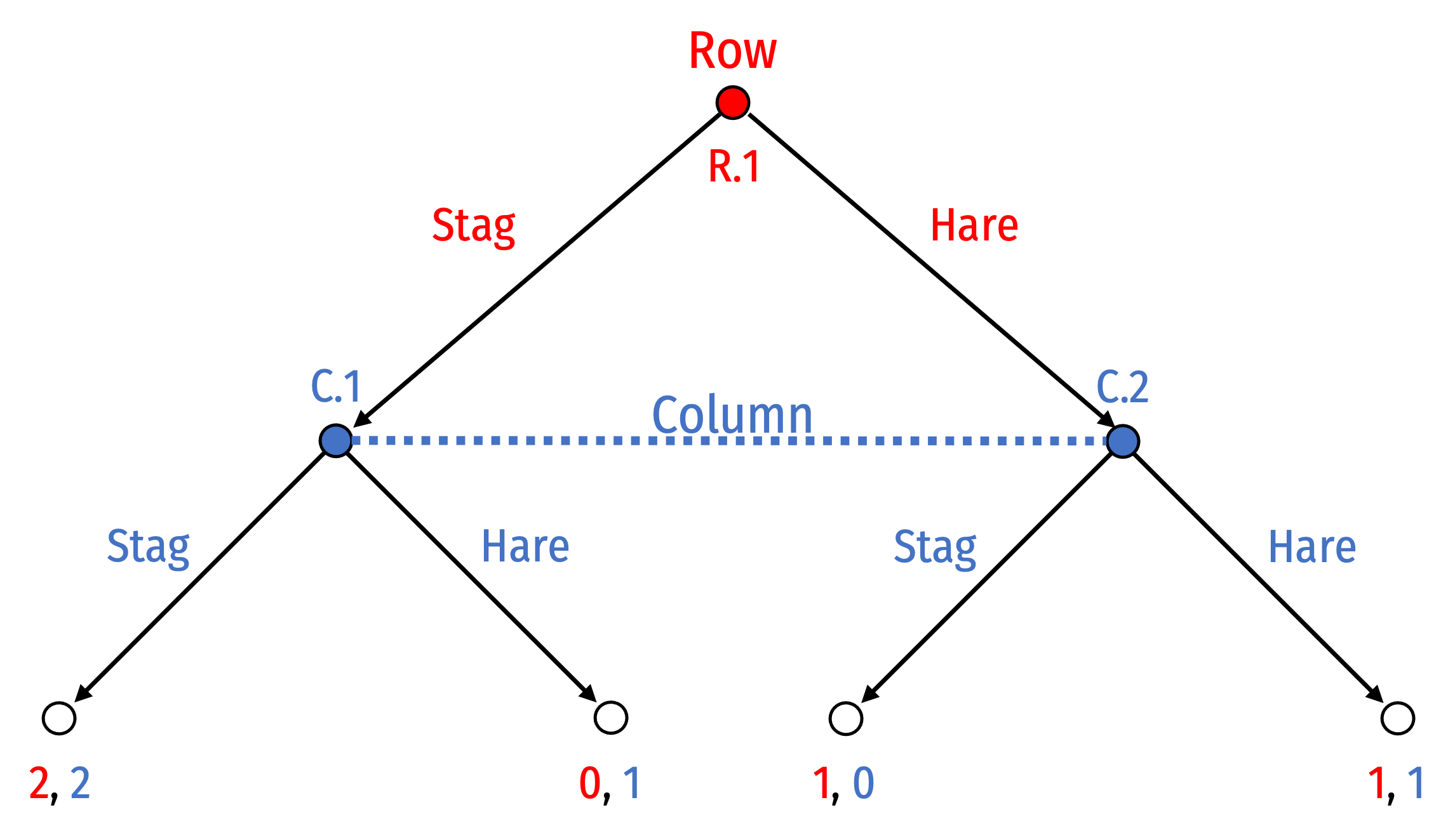
We can model it in extensive form with imperfect information
- Let Row move first (order really doesn't matter with symmetric payoffs)
Row’s move is hidden from Column:
- Can't distinguish between the history where Row chose Stag and the history where Row chose Hare.
Simultaneous Games and Info Sets
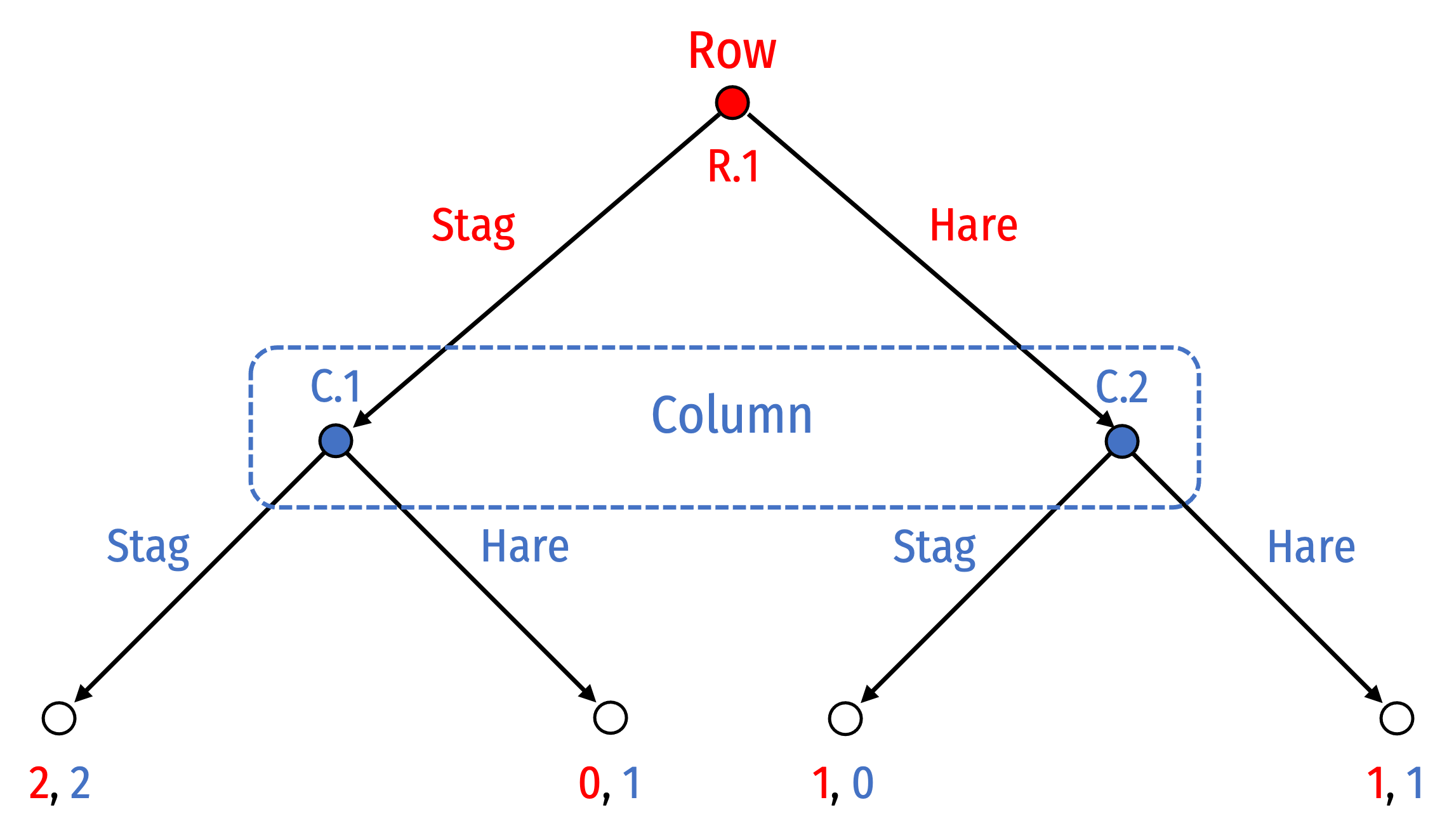
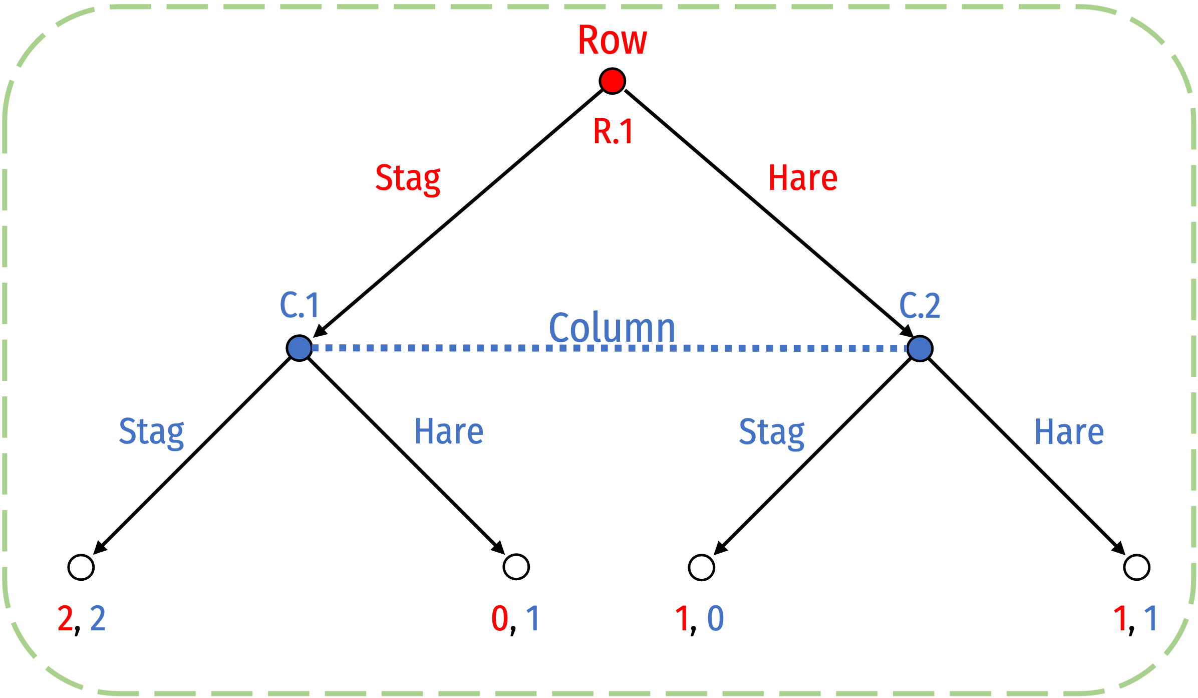
Information set (dotted line/oval connecting decision nodes) for Column ⟹ can’t distinguish between histories of Stag or Hare
Column doesn’t know if they are deciding at node C.1 or C.2 (whether Row has played Stag or Hare)

Simultaneous Games and Info Sets
Information set (dotted line/oval connecting decision nodes) for Column ⟹ can’t distinguish between histories of Stag or Hare
Column doesn’t know if they are deciding at node C.1 or C.2 (whether Row has played Stag or Hare)
Simultaneous Games: No Mover Advantage

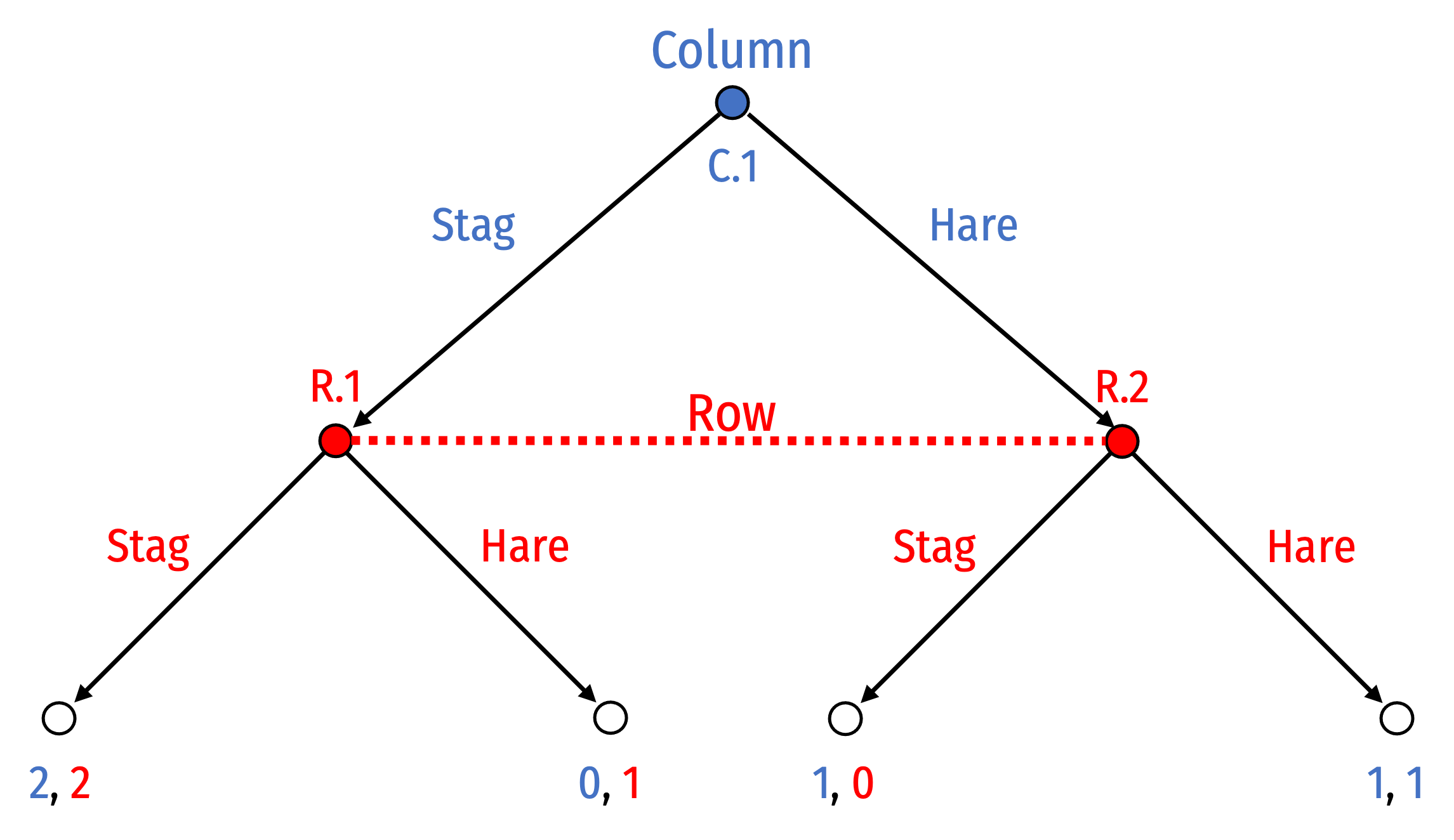
- Note changing who moves first here makes no difference on the game, since “second-mover” still does not know what “first-mover” chooses!
Strategies and Information Sets
Strategies available to player within an information set must be the same across all decision nodes/histories
If they are different, player can tell which history they are on given the unique strategies available to them
- Column would clearly know if they are at node C.1 or C.2 since strategies available are different!
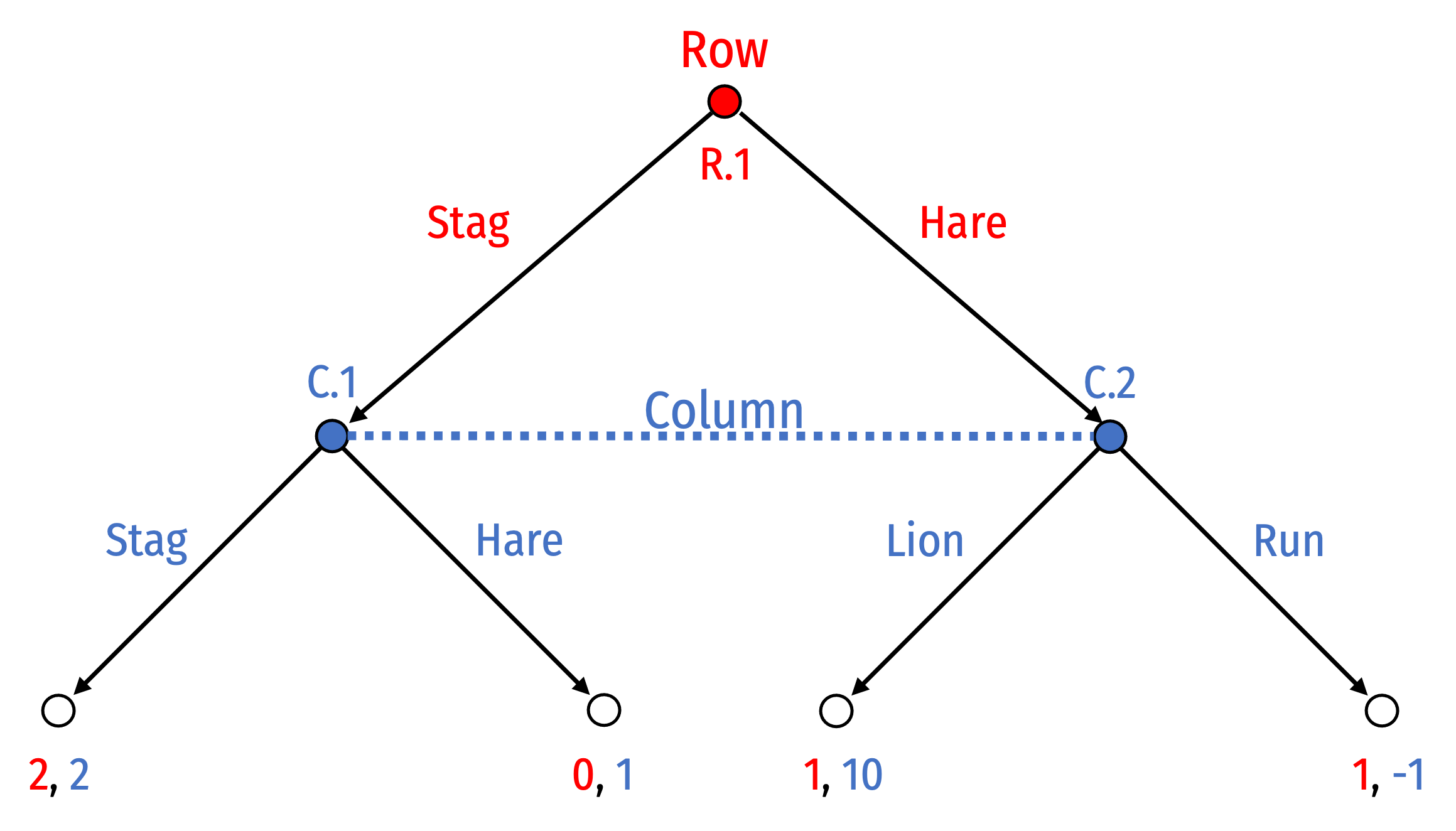
This is not a valid game
Strategies and Information Sets
Furthermore, Column must play the same strategy across the decision nodes
- (i.e. always Stag or always Hunt) at both (C.1 and C.2)
- Can’t play (Stag, Hare) or (Hare, Stag) at (C.1,C.2)
Again, doesn’t know what decision node they are actually deciding at

Strategies and Information Sets
Clarify what we mean by strategy: a complete plan of action of all the decisions a player will make at every possible information set
- (rather than merely every decision node)
Until now, information sets have consisted of a single decision node (“singleton”)

Perfect Information
We can now more precisely define perfect information: no information sets contain multiple decision nodes (are all “singleton” nodes)
Individual can differentiate between histories of game at each decision node
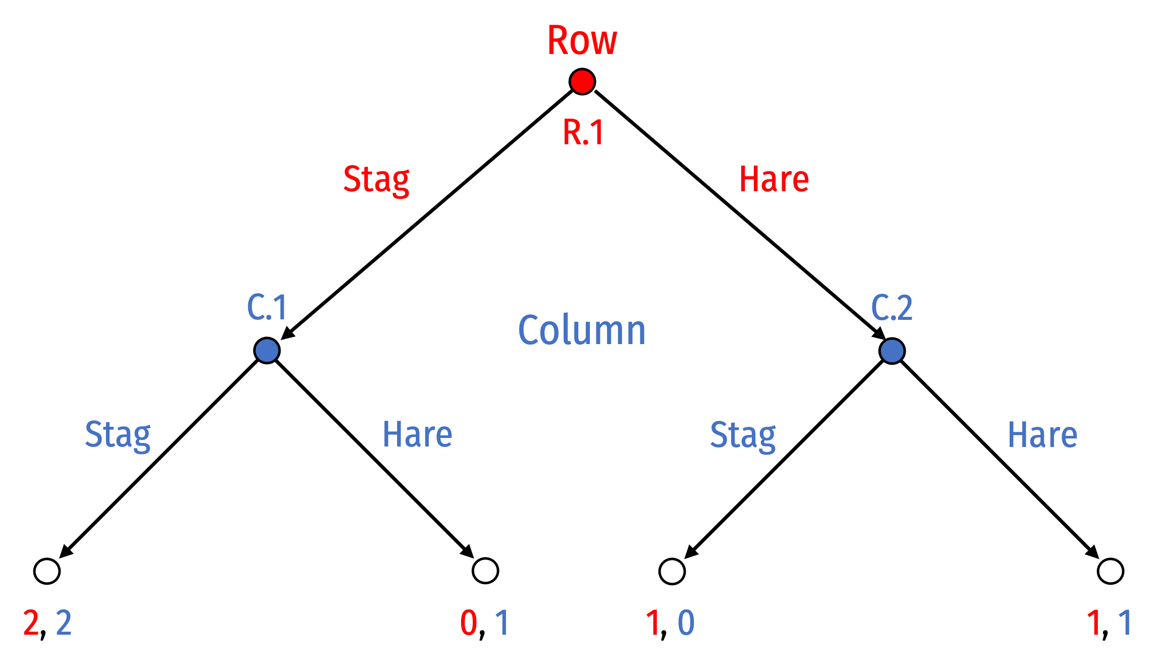
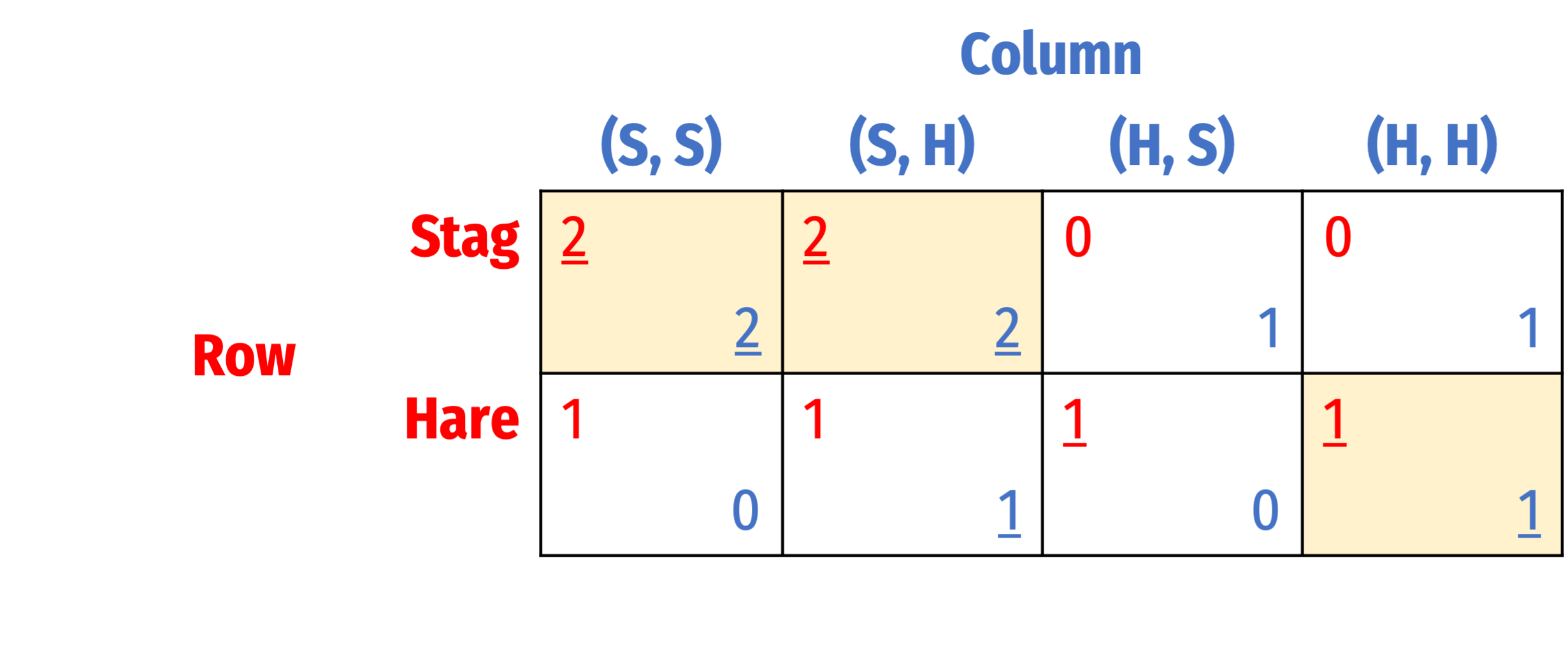
Stag Hunt with Perfect Information
With perfect information, Column’s strategies can be conditional on what Row plays
- (Stag, Stag)
- (Stag, Hare)
- (Hare, Stag)
- (Hare, Hare)
Each information set is a singleton (i.e. nodes C.1 and C.2 each contain a separate information set)

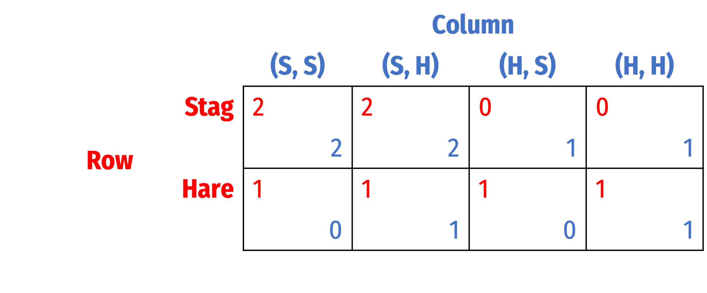
Stag Hunt with Perfect Information
- Using normal form, three Nash equilibria with perfect information:
- {Stag, (Stag, Stag)}
- {Stag, (Stag, Hare)}
- {Hare, (Hare, Hare)}

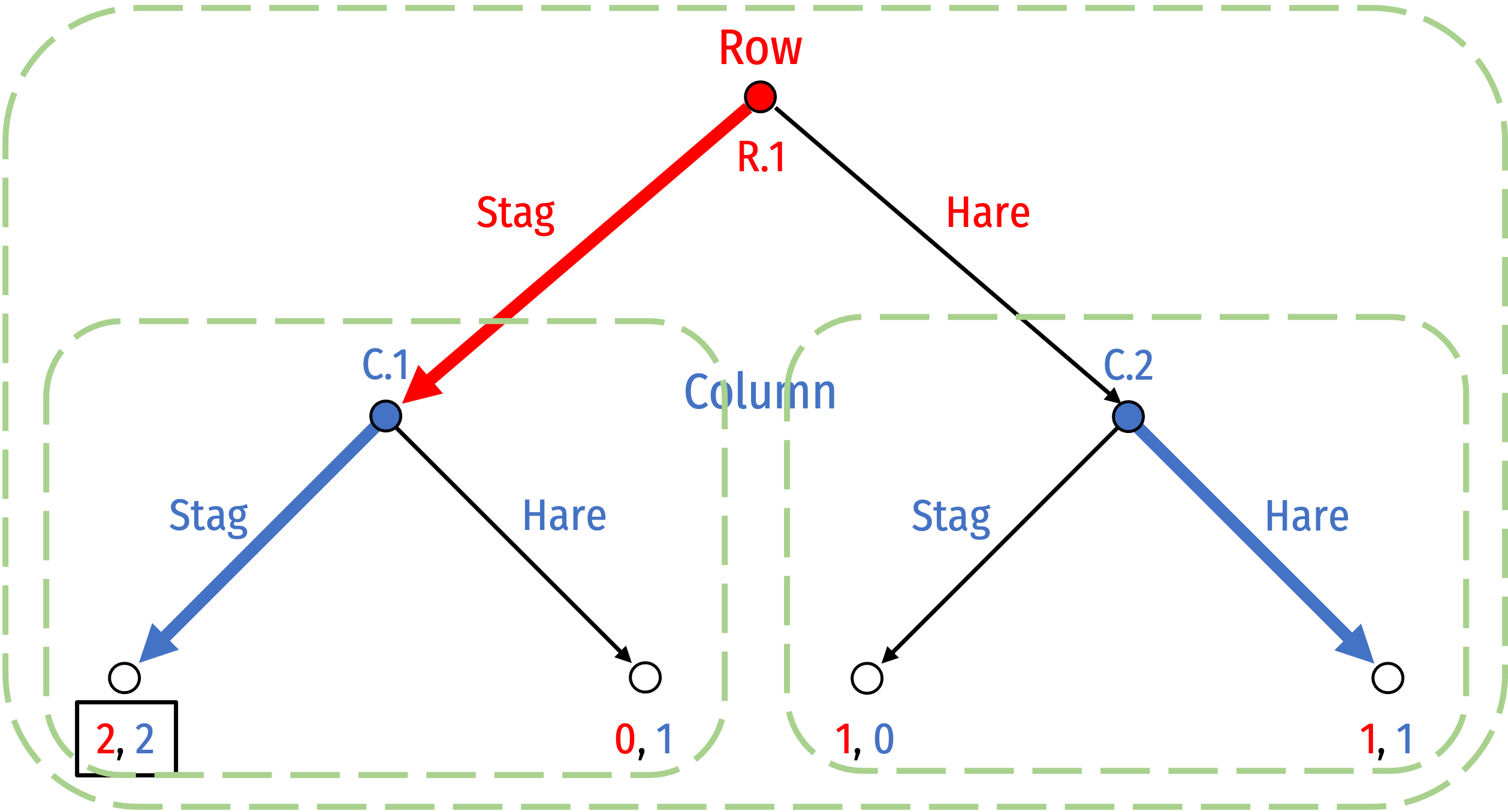
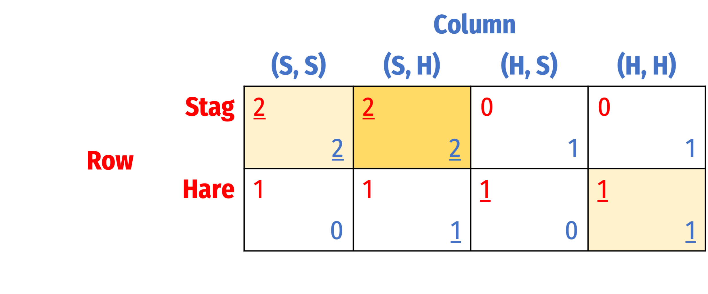
Stag Hunt with Perfect Information
- Using normal form, three Nash equilibria with perfect information:
- {Stag, (Stag, Stag)}
- {Stag, (Stag, Hare)}
- {Hare, (Hare, Hare)}
- Only #2 {Stag, (Stag, Hare)} is subgame perfect
Imperfect Information and Subgame Perfection
With imperfect information, some information sets contain multiple decision nodes
A subgame must contain all nodes in the information set, cannot “break” information sets
- Nodes 2.1 and 2.2 do not initiate subgames (breaks information sets)
- The only subgame possible is the overall game itself (contains all nodes in information set)
We cannot use subgame perfection as a solution concept here
Imperfect Info. May Imply A Simultaneous Game
Column cannot play any conditional strategies depending on what Row does
- Can’t know what Row will play!
- Must choose an unconditional strategy to always play Stag or Hare
All we can do is solve the game via strategic form as usual
Incomplete Information
Incomplete Information
Even in games with imperfect information (e.g. simultaneous games), we have assumed information was complete
- Players know the rules, strategies available, and the payoffs to each player
Source of uncertainty was strategic: players didn’t know the history of the game (moves made by other players)

Incomplete Information
Now consider games with incomplete information
- Players don’t know something about the game
- Common example: what the payoffs to the other player are (but know your own)
Textbook calls this external uncertainty: the game is not fully clear due to some undetermined external factors

External Uncertainty: Playing with Nature
We can deal with external uncertainty by including Nature as a player
Nature has no strategic interest in the outcomes (has no payoff and no objectives)
Really just a metaphor for rolling (possibly weighted) dice

External Uncertainty: Simple Example
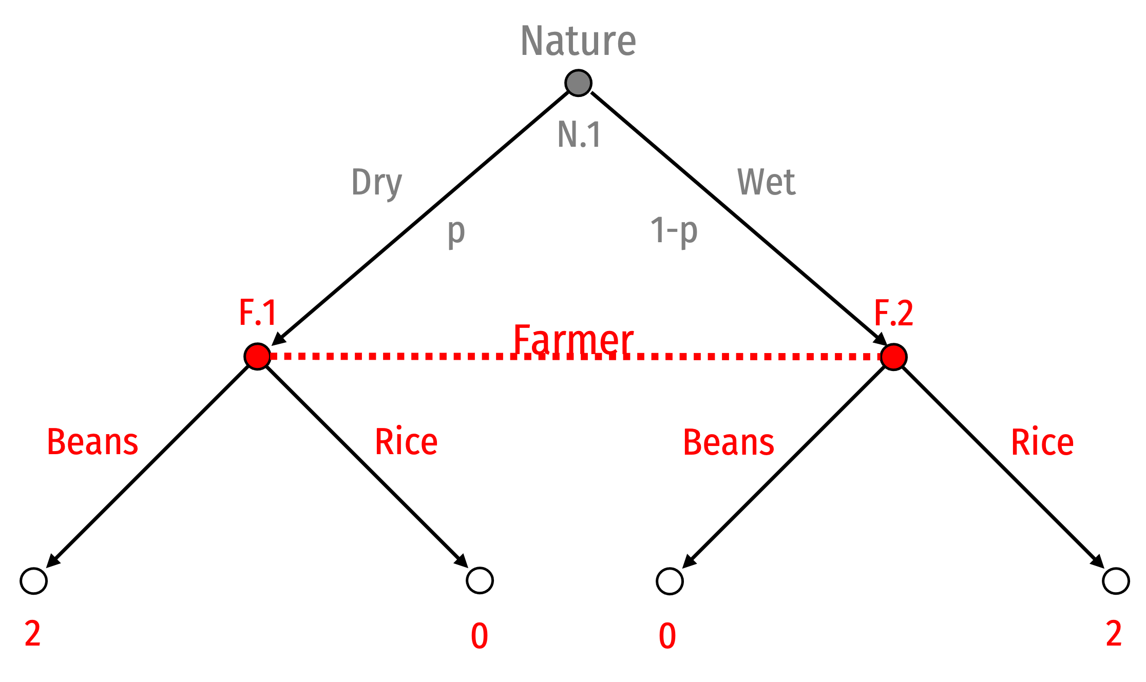
Consider a Farmer who (ignoring competition) must determine what crops to plant: Beans, which do better in dry seasons; or Rice which does better in wet seasons
Let Nature decide what the weather this season will be
- With some probability p, Nature will “choose” a wet season
Farmer can’t know what Nature chose
External Uncertainty: Simple Example
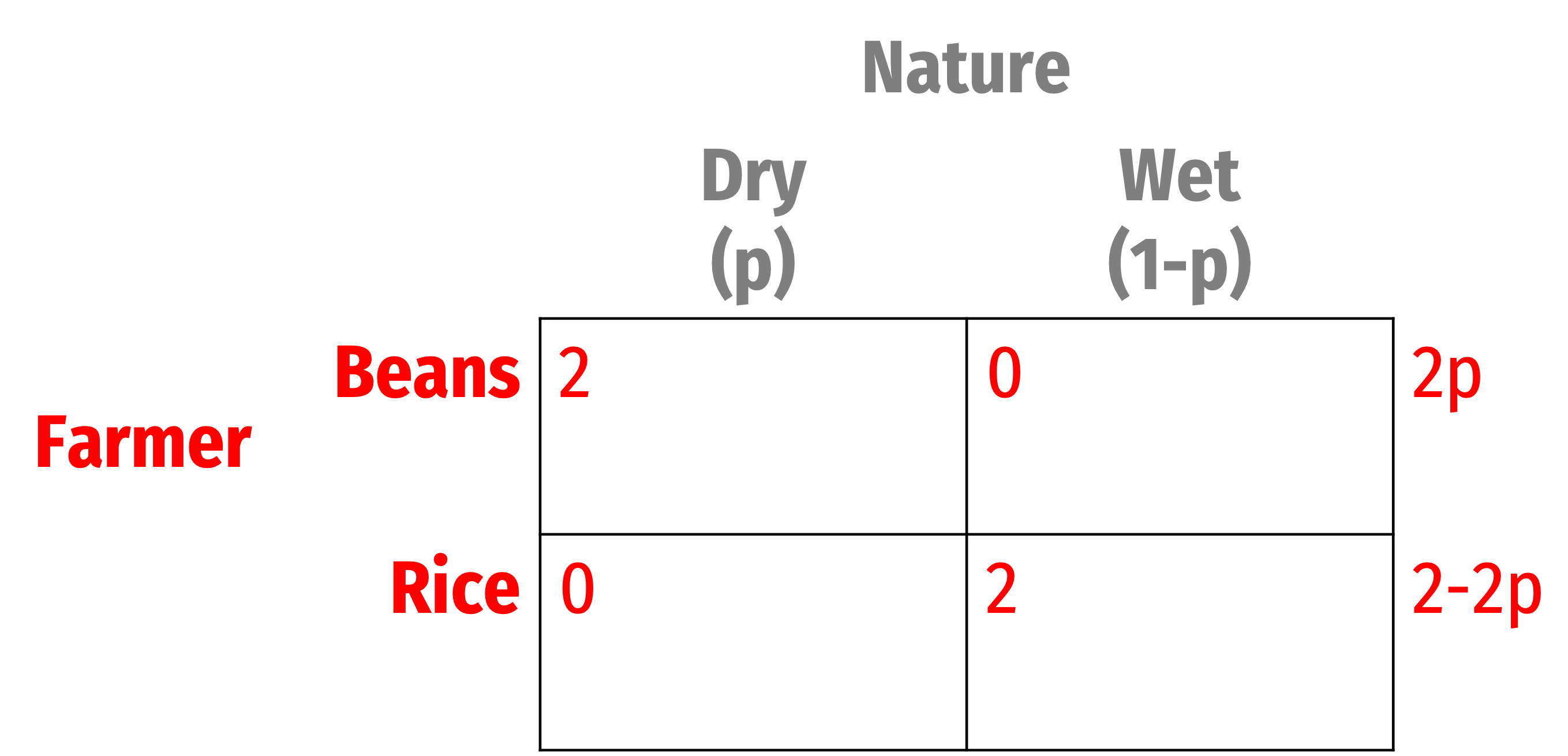
Farmer must maximize expected payoff
Consider a mixed strategy “against” Nature
External Uncertainty: Simple Example
Farmer must maximize expected payoff
Consider a mixed strategy “against” Nature
E[Beans]=E[Rice]2p=2−2pp⋆=0.50
- If p>0.50, Farmer should plant Beans
- If p<0.50, Farmer should plant Rice

External Uncertainty: Simple Example
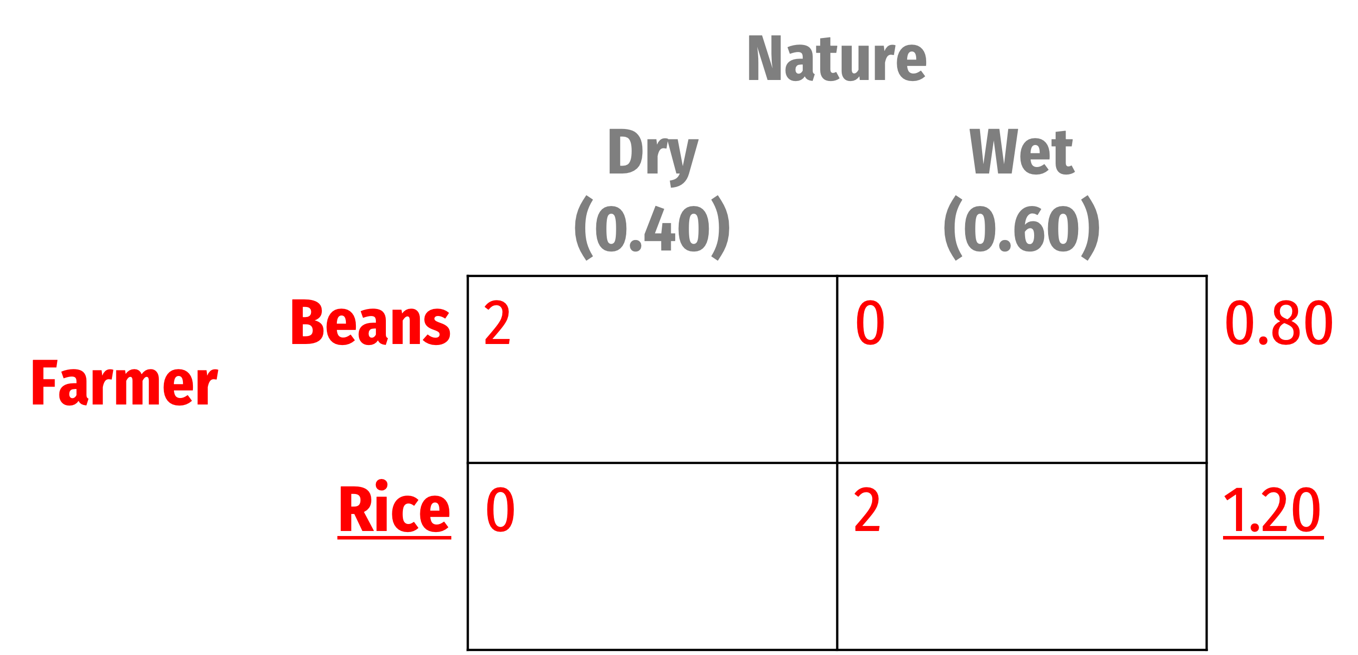
Now suppose Farmer can estimate (based on experience, forecasts, etc) p to be 0.40
Now Farmer has a pure strategy “against” Nature
E[Beans]<E[Rice](0.40)2+(0.60)0+<(0.40)0+(0.60)20.80<1.20
- Definitely plant Rice
External Uncertainty: Simple Example
- Key here is Farmer’s beliefs about p

Asymmetric Information & Simultaneous Bayesian Games
Asymmetric Information
A particular type of incomplete information is asymmetric information, where players might not know all relevant information about others
- Other player’s strategies, payoffs, preferences, or “type”
Typically, one player has important private information about themself that other players are not privy to
- e.g. Player 2 knows their “type” but Player 1 does not know Player 2’s type

Asymmetric Information

John C. Harsanyi
1920—2000
Economics Nobel 1994
“[T]he original game can be replaced by a game where nature first conducts a lottery in accordance with the basic probablity distribution, and the outcome of this lottery will decide which particular subgame will be played, i.e., what the actual values of the relevant parameters will be in the game. Yet each player will receive only partial information about the outcome of the lottery, and about the values of these parameters,” (p.159).
Asymmetric Information

John C. Harsanyi
1920—2000
Economics Nobel 1994
“In such a game player 1's strategy choice will depend on what he expects (or believes) to be player 2's payoff function U2, as the nature of the latter will be an important detemunant of player 2's behavior in the game...If we follow the Bayesian approach and represent the players' expectations or beliefs by subjective probability distributions, then player 1's first-order expectation will have the nature of a subjective probability distribution P11(U2) over all alternative payoff functions U2 that player 2 may possibly have. Likewise, player 2's first-order expectation will be a subjective probability distribution P12(U1) over all alternative payoff functions U1 that player 1 may possibly have,” (pp.163—164).
Asymmetric Information

John C. Harsanyi
1920—2000
Economics Nobel 1994
“The purpose of this paper is to suggest an alternative approach to the analysis of games with incomplete information. This approach will be based on constructing, for any given game [of incomplete information], some game [of complete information] game-theoretically equivalent to [the first game].” (pp.164—165).
“Thus, our approach will basically amount to replacing a game G involving incomplete information, by a new game G⋆ which involves complete but imperfect information, yet which is, as we shall argue, essentially equivalent to G from a game-theoretical point of view,” (p.166).
Asymmetric Information

John C. Harsanyi
1920—2000
Economics Nobel 1994
“Accordingly, we define a [game of incomplete information] G where every player j knows the strategy spaces Si of all players i=1,⋯,j,⋯n but where, in general, he does not know the payoff functions Ui of these players i=1,⋯,j,⋯n,” (p.166).
Asymmetric Information
Players have beliefs about other players’ strategies & payoffs according to a probability distribution
- Harsanyi shows it’s sufficient to assume players have a “type”
Shows that for every game of incomplete information, there are equivalent (sub-)games with complete (but imperfect) information
“Bayesian” since players assumed to update their beliefs according to Bayes’ rule (more on that next time)

Asymmetric Information
- Until now, our definition of a game (with complete information) has consisted of:
- Players
- Strategies
- Payoffs (jointly determined by players’ chosen strategies)
Asymmetric Information
- With a game of incomplete information a game consists of:
- Players
- Types of players
- Common prior beliefs about players
- Strategies
- Strategies conditioned on beliefs about player types
- Payoffs (jointly determined by players’ chosen strategies)
- Payoffs depend on types

Bayesian Simultaneous Games
A new class of Bayesian games due to the role of information and beliefs
We will consider simultaneous games first, then sequential games later
Bayesian Nash equilibrium (BNE): set of strategies, one for each (type of) player where no (type of) player wants to change given what the others are doing
- i.e. each (type of) player is playing a best response

Bayesian Nash Equilibria
- Two categories of equilibria in Bayesian games (with different players)
- Pooling equilibrium: all types of players play the same strategy
- Separating equilibrium: different types of players play different strategies

Bayesian Game Example
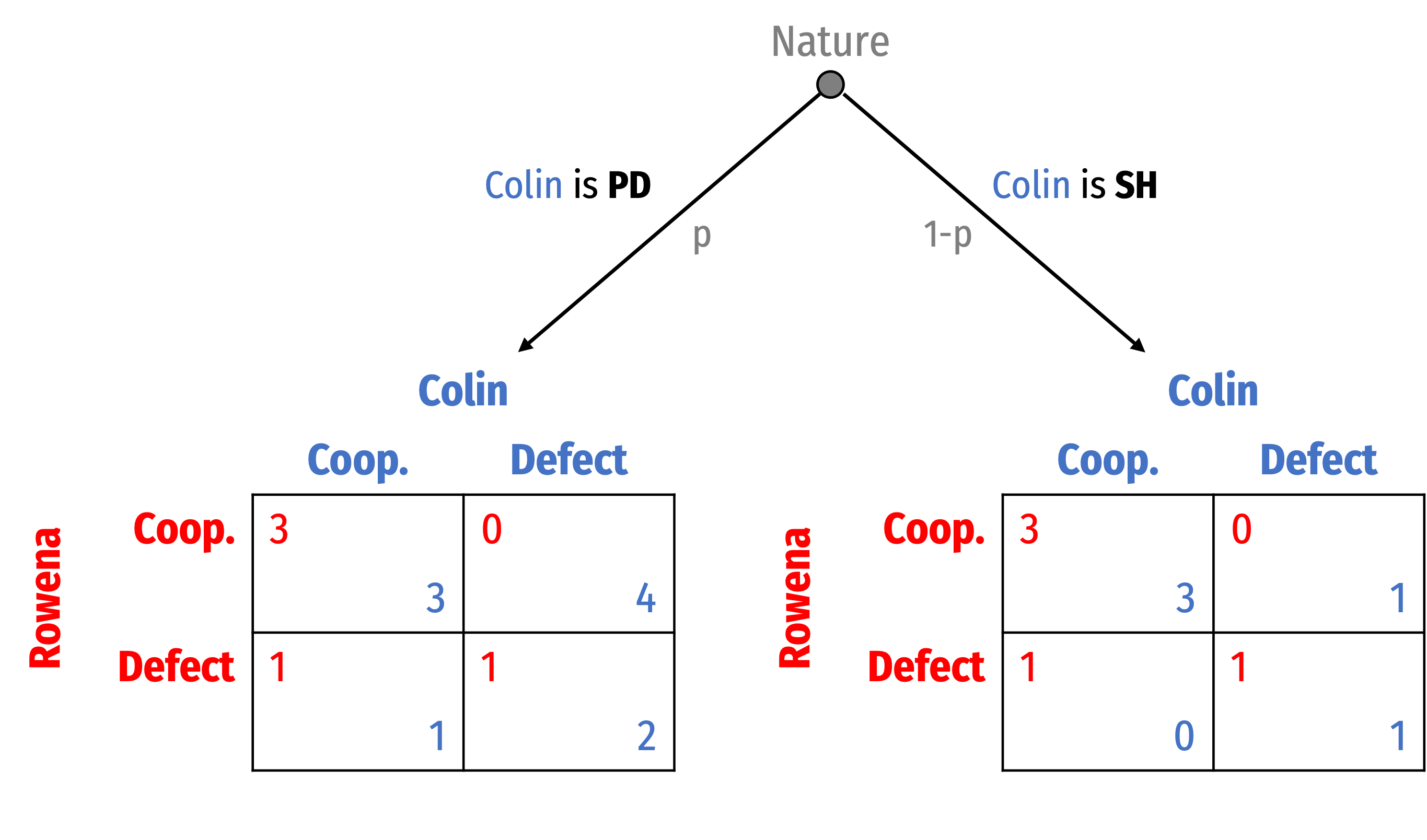
Rowena and Colin play where they can each Cooperate or Defect
Suppose Colin could be one of two types:
- Prisoners’ Dilemma-type payoffs:
(C, D) ≻ (C, C) ≻ (D, D) ≻ (D, C)
- Stag Hunt-type payoffs:
(C, C) ≻ (D, D) ∼ (C, D) ≻ (D, C)
Rowena has Stag Hunt-type payoffs
(C, C) ≻ (D, D) ∼ (D, C) ≻ (C, D)

Interpreting Nature in the Example
The identity of the other player is known, but their preferences are unknown
- Rowena know she is playing with Colin, but doesn’t know if he has PD or SH preferences
- Nature whispers to Colin his type, and Rowena has to figure it out
Nature selects Colin from a population of potential player types
- Rowena knows she will play with another player, but doesn’t know if s/he is playing PD or SH, Nature decides

Bayesian Game Example
- Rowena must choose between two strategies, Cooperate or Defect

Bayesian Game Example
Rowena must choose between two strategies, Cooperate or Defect
If she plays Cooperate, for example:
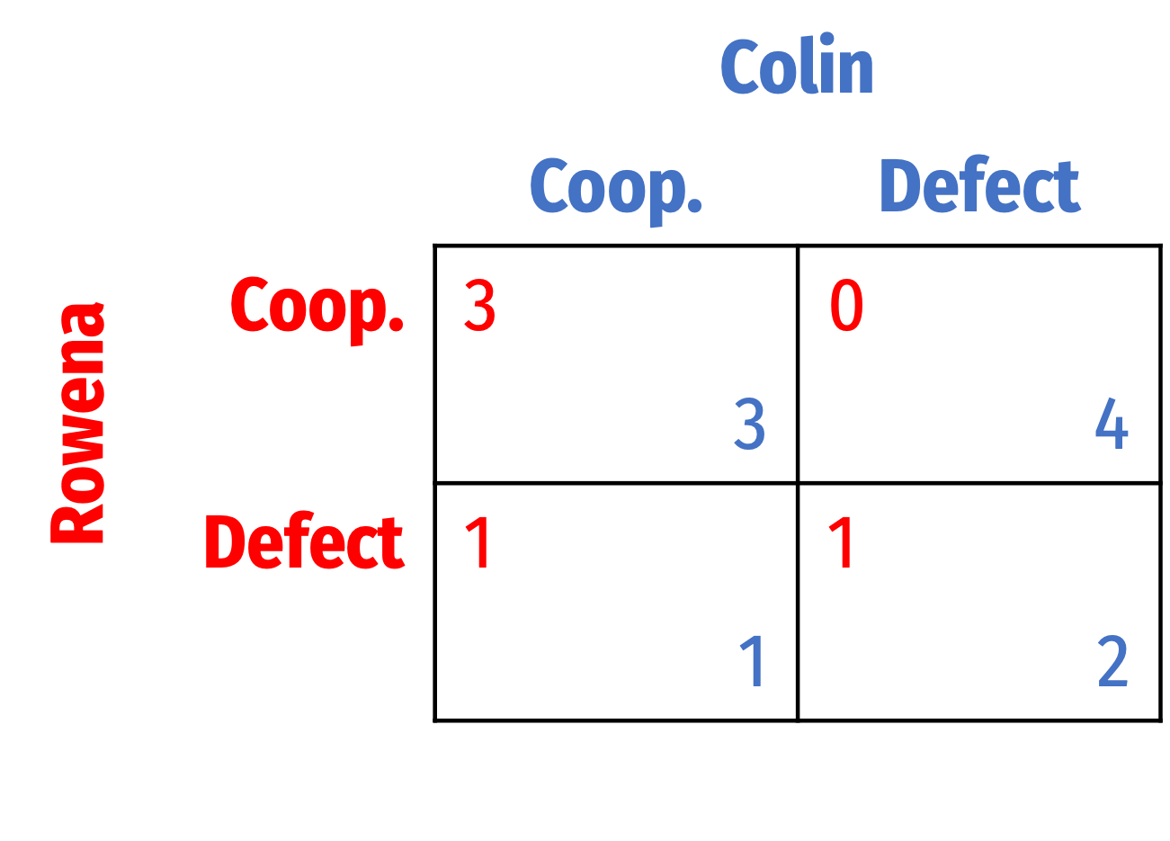
- A SH-type Colin will want to Cooperate, giving her 3
- A PD-type Colin will want to Defect, giving her 0
Rowena will have to consider her own expected payoff of playing each strategy against both types of Colin
- Depends on her beliefs about p!

Bayesian Game Example
Simple example, suppose (she believes) p=1.00, Rowena is for sure playing against a PD-type Colin
Game simplifies to a game of complete imperfect information
Pure strategy Nash equilibrium: (Defect, Defect)
- Colin has dominant strategy to Defect
- Rowena’s best response is to Defect
Exploring BNE in Bayesian Game Example
- Different potential Bayesian Nash equilibrium (BNE):
1) Pooling equilibria: both types of Colin play the same strategy
- Scenario I: Colin-types both Cooperate
- Scenario II: Colin-types both Defect

Exploring BNE in Bayesian Game Example
- Different potential Bayesian Nash equilibrium (BNE):
2) Separating equilibria: each type of Colin plays a different strategy
- Scenario III: PD-type Colin plays Cooperate; SH-type Colin plays Defect
- Scenario IV: PD-type Colin plays Defect; SH-type Colin plays Cooperate

Pooling Eq. I: Both Types Cooperate (?)
Pooling equilibrium I: both Colin-types play Cooperate, i.e. (C,C)
❌ This is impossible: PD-type Colin has a dominant strategy to Defect
- Would switch from Cooperate to Defect

Pooling Eq. II: Both Types Defect (?)
Pooling equilibrium II: both Colin-types play Defect, i.e. (D,D)
Rowena maximizes her expected payoff against unknown Colin-type playing Defect

Pooling Eq. II: Both Types Defect (?)
Pooling equilibrium II: both Colin-types play Defect, i.e. (D,D)
Rowena maximizes her expected payoff against unknown Colin-type playing Defect
E[Cooperate]=0p+0(1−p)E[Cooperate]=0

Pooling Eq. II: Both Types Defect (?)
Pooling equilibrium II: both Colin-types play Defect, i.e. (D,D)
Rowena maximizes her expected payoff against unknown Colin-type playing Defect
E[Cooperate]=0p+0(1−p)E[Cooperate]=0
E[Defect]=1p+1(1−p)E[Defect]=1
- Rowena will always play Defect

Pooling Eq. II: Both Types Defect (?)
Pooling equilibrium II: both Colin-types play Defect. i.e. (D,D)
✅ This is a valid Bayesian Nash Equilibrium: {Defect, (Defect, Defect)}
- Where Colin’s strategies are denoted for (PH-type Colin, SH-type Colin)

Separating Eq. I: PD-Type Coops; SH-Type Defects (?)
- Separating equilibrium I: PD-type Colin plays Cooperate; SH-type Colin plays Defect, i.e. (C,D)

Separating Eq. I: PD-Type Coops; SH-Type Defects (?)
Separating equilibrium I: PD-type Colin plays Cooperate; SH-type Colin plays Defect, i.e. (C,D)
❌ This is impossible: PD-type Colin has a dominant strategy to Defect
- Would switch from Cooperate to Defect

Separating Eq. II: PD-Type Defects; SH-Type Coops. (?)
Separating equilibrium II: PD-type Colin plays Defect; SH-type Colin plays Cooperate, i.e. (D,C)
Rowena maximizes her expected payoff against unknown Colin-type:

Separating Eq. II: PD-Type Defects; SH-Type Coops. (?)
Separating equilibrium II: PD-type Colin plays Defect; SH-type Colin plays Cooperate, i.e. (D,C)
Rowena maximizes her expected payoff against unknown Colin-type:
E[Cooperate]=0p+3(1−p)E[Cooperate]=3−3p

Separating Eq. II: PD-Type Defects; SH-Type Coops. (?)
Separating equilibrium II: PD-type Colin plays Defect; SH-type Colin plays Cooperate, i.e. (D,C)
Rowena maximizes her expected payoff against unknown Colin-type:
E[Cooperate]=0p+3(1−p)E[Cooperate]=3−3p
E[Defect]=1p+1(1−p)E[Defect]=1

Separating Eq. II: PD-Type Defects; SH-Type Coops. (?)
Separating equilibrium II: PD-type Colin plays Defect; SH-type Colin plays Cooperate, i.e. (D,C)
Rowena maximizes her expected payoff against unknown Colin-type:
E[Cooperate]=E[Defect]3−3p=1p=23

Separating Eq. II: PD-Type Defects; SH-Type Coops. (?)
Separating equilibrium II: PD-type Colin plays Defect; SH-type Colin plays Cooperate, i.e. (D,C)
When p>23, Rowena should play Defect ✅
- When p<23, Rowena should play Cooperate
- Here, a SH-type Colin would want to switch from Cooperate to Defect; this would not be a BNE ❌

Bayesian Nash Equilibria
- Our two possible Bayesian Nash equilibria (BNE):
{Defect, (Defect, Defect)}, a pooling equilibrium
{Defect, (Cooperate, Defect)}, a separating equilibrium, if p>23
- If p<23, no equilibrium
- Note that these depend on Rowena’s beliefs about p!
- Next...why these are Bayesian games
